# Import required libraries 

import numpy as np
import pandas as p
import tensorflow as tf

import matplotlib.pyplot as plt

from tensorflow.keras.datasets import mnist
from tensorflow.keras import layers, models, optimizers, regularizers
from scipy.stats import norm
%matplotlib inline 

# Get a subset of the mnist data
x_train, x_test = np.load('mnist_mini_train.npy'), np.load('mnist_mini_test.npy')

# Function to 
# 1. Change dimensions
# 2. Change datatype
def binary_preprocess(imageset):
    imageset = imageset.reshape(imageset.shape[0],28,28,1)/255.
    return np.where(imageset > .5, 1.0,0.0).astype('float32')

# Pre-processed images to satisfy the Independent Bernoulli condition
x_train_images = binary_preprocess(x_train)
x_test_images = binary_preprocess(x_test)

# Dataset object to get a mini-batch
batch_size = 100
train_size = x_train_images.shape[0]
latent_size = 2
input_shape = (28,28,1)

# Model encoder architecture 
encoder = tf.keras.Sequential(
          [
            tf.keras.layers.InputLayer(input_shape=(28,28, 1)),
            tf.keras.layers.Flatten(),
            tf.keras.layers.Dense(128,activation='relu'),
            tf.keras.layers.Dense(32,activation='relu'),
            # No activation
            tf.keras.layers.Dense(4),
        ]
    )

# Model decoder architecture 
decoder = tf.keras.Sequential(
        [
            tf.keras.layers.InputLayer(input_shape=(2,)),
            tf.keras.layers.Dense(32, activation='relu'),
            tf.keras.layers.Dense(128, activation='relu'),
            tf.keras.layers.Dense(784,activation='sigmoid'),
            tf.keras.layers.Reshape((28,28,1))
        ]
    )

# Encoding step
# Note: We use logvariance instead of variance 

# Get the mean and the logvariance
def encode(encoder,x):
    activations = encoder(x)
    mean, logvariance = tf.split(activations,num_or_size_splits=2,axis=1)
    return mean,logvariance

# Reparametrization step
def sample(mu, logvariance):
    
    # Here we sample from N(0,1)
    e = tf.random.normal(shape=mu.shape)
    return e * tf.exp(logvariance/2) + mu

# Combine the autoencoder
def autoencoder(encoder,decoder,x):
    mean,logvariance = encode(encoder,x)
    z = sample(mean,logvariance)
    output = decoder(z)
    return output

# Quick way to get the log likelihood of a normal distribution
def log_normal_pdf(value, mean, logvariance, raxis=1):
    log_2pi = tf.math.log(2. * np.pi)
    logpdf = -(logvariance + log_2pi + (value - mean)**2. * tf.exp(logvariance))/2
    return tf.reduce_sum(logpdf,axis=1)

    

# Loss over the assumed distribution(qz_x) and the prior(pz)
def analytical_kl(encoder,x):
    mean, logvariance = encode(encoder,x)
    # tf.reduce_sum is over the hidden dimensions
    lossval = tf.reduce_sum(-0.5*(1 + logvariance - tf.square(mean) - tf.exp(logvariance)),axis=-1)
    return tf.reduce_mean(lossval)

# This is now binary cross entropy
# Crucially, observe that we sum across the image dimensions
# and only take the mean in the images dimension
def reconstruction_loss(encoder,decoder,x):
    x_pred = autoencoder(encoder,decoder,x)
    loss = tf.keras.losses.binary_crossentropy(x,x_pred)
    # tf.reduce_sum is over all pixels and tf.reduce_mean is over all images
    return tf.reduce_mean(tf.reduce_sum(loss,axis=[1,2]))

# Instantiate an optimizer with a learning rate
optimizer = tf.keras.optimizers.RMSprop(learning_rate=1e-3)

# Define number of epochs
num_epochs = 300


# Loop over the required number of epochs
for i in range(num_epochs):
    for j in range(int(train_size/batch_size)):
        
        # Randomly choose a minitbatch
        x_train_batch = x_train_images[np.random.choice(train_size,batch_size)]
        
        # Open the gradienttape to map the computational graph
        with tf.GradientTape(persistent=True) as t:
            
            decoder_output = autoencoder(encoder,decoder,x_train_batch)

            L1 = reconstruction_loss(encoder,decoder,x_train_batch)
            L2 = analytical_kl(encoder,x_train_batch)
            # Adding the reconstruction loss and KL divergence
            loss = L1 + L2
            
        # We take the gradients with respect to the decoder    
        gradients1 = t.gradient(loss, decoder.trainable_weights)
        # We take the gradients with respect to the encoder        
        gradients2 = t.gradient(loss, encoder.trainable_weights)
        
        # We update the weights of the decoder
        optimizer.apply_gradients(zip(gradients1, decoder.trainable_weights))
        # We update the weights of the decoder        
        optimizer.apply_gradients(zip(gradients2, encoder.trainable_weights))
    
    # We display the loss after every 10 epochs
    if i+1%10==0:
        print(f'Loss at epoch {i+1} is {loss:.2f}, KL Divergence is {L2:.2f}')

# We choose a text sample index
test_sample = 10

# We make a prediction
# NOTE: Since we did not add a sigmoid activation,
# We must specify it now to convert logits to probabilities
pred = autoencoder(encoder,decoder,x_test_images[test_sample:test_sample+1])

# We make class predictions for each pixel (ON or OFF)
pred = np.where(pred>0.5,1,0)
pred = pred.squeeze()
pred.shape

# We plot the reconstruction with the true input 
fig, ax = plt.subplots(1,2)
ax[0].imshow(x_test_images[test_sample].squeeze(),cmap='gray')
ax[1].imshow(pred,cmap='gray')
ax[0].set_title('True image',fontsize=14)
ax[1].set_title('Reconstruction',fontsize=14);
ax[0].axis('off');
ax[1].axis('off');
plt.show()

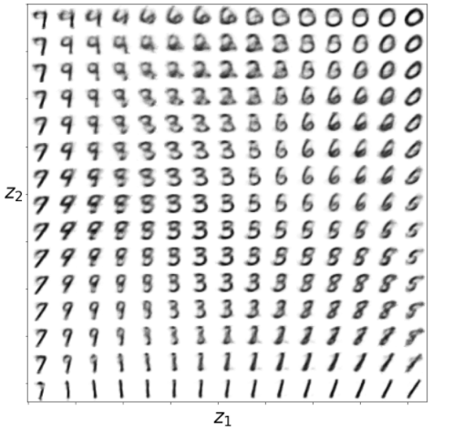
# display a 2D manifold of the digits
n = 15  # figure with 15x15 digits
digit_size = 28

latent_dim = 2

# linearly spaced coordinates on the unit square were transformed
# through the inverse CDF (ppf) of the Gaussian to produce values
# of the latent variables z, since the prior of the latent space
# is Gaussian

z1 = norm.ppf(np.linspace(0.01, 0.99, n))
z2 = norm.ppf(np.linspace(0.01, 0.99, n))
z_grid = np.dstack(np.meshgrid(z1, z2))

x_pred_grid = tf.sigmoid(decoder.predict(z_grid.reshape(n*n, latent_dim))).numpy() \
                     .reshape(n, n, digit_size, digit_size)

fig, ax = plt.subplots(1,1, figsize=(10,10))
ax.imshow(np.block(list(map(list, x_pred_grid))),cmap='binary')
# ax.axis('off')
ax.set_xlabel('$z_1$  ', fontsize=32)
ax.set_ylabel('$z_2$   ', fontsize=32,rotation=0)
ax.set_xticklabels('')
ax.set_yticklabels('')
plt.tight_layout()