Title
Autoencoders on Iris data
Description :
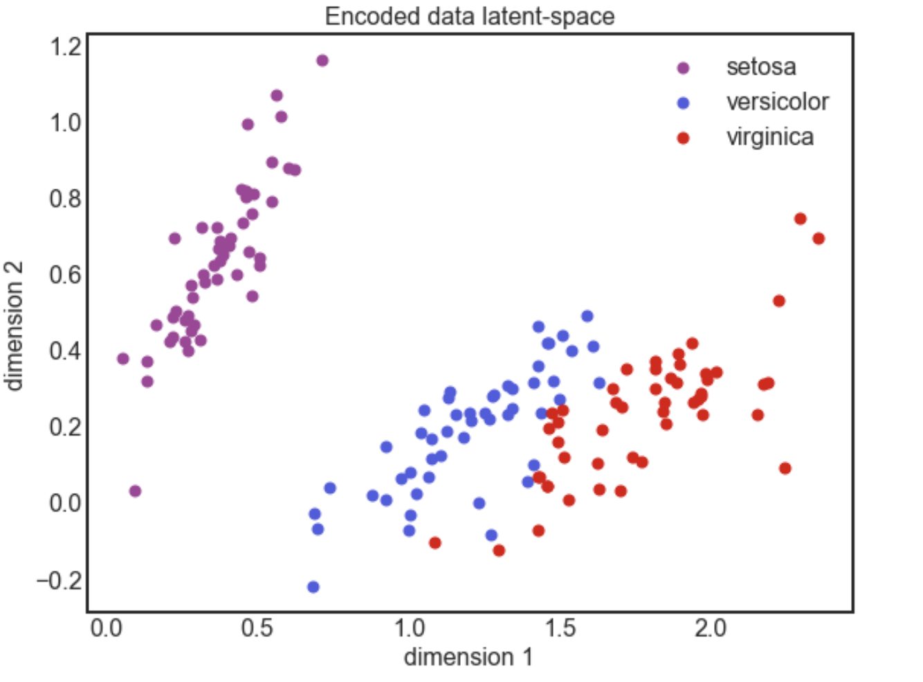
The goal of this exercise is to visualize the latent-space for the autoencoder trained on the IRIS dataset.
Instructions:
- Load the IRIS dataset with the
load_iris()function provided by keras. - Load the predictors as the variable
Xand the targets as the variabley. - Make a basic autoencoder model (Encoder - Decoder) as follows:
- Map encoder to a latent (hidden) space - input dimension is 4 and output dimension is 2.
- Use the decoder to reconstruct - input dimension is 2 and output dimension is 4.
- Make the final
autoencodermodel with the help of the keras functional API - Compile the model with an appropriate
optimizerandloss. - Train the model for several epochs and save the training into a variable
history. - Plot the
lossandvalidation_lossover the epochs. - Finally plot the latent space representation along with the clusters using the
plot3clusters()function. This plot will look similar to the one given above.
Hints:
keras.compile() Compiles the layers into a network.
keras.Sequential() Models a sequential neural network.
keras.Dense() A regular densely-connected NN layer.
tf.keras.Input() Used to instantiate a Keras tensor.
In [1]:
# Import the necessary libraries
import pandas as pd
import numpy as np
from sklearn.datasets import load_iris
from sklearn.preprocessing import MinMaxScaler
from sklearn.decomposition import PCA
from matplotlib import pyplot as plt
%matplotlib inline
import tensorflow as tf
In [2]:
# Run this cell for more readable visuals
large = 22; med = 16; small = 10
params = {'axes.titlesize': large,
          'legend.fontsize': med,
          'figure.figsize': (16, 10),
          'axes.labelsize': med,
          'axes.titlesize': med,
          'axes.linewidth': 2,
          'xtick.labelsize': med,
          'ytick.labelsize': med,
          'figure.titlesize': large}
plt.style.use('seaborn-white')
plt.rcParams.update(params)
%matplotlib inline
In [63]:
#Load Iris Dataset
iris = load_iris()

# Get the predictor and response variables
X = iris.data
y = iris.target

# Get the Iris label names
target_names = iris.target_names
print(X.shape, y.shape)

# Standardize the data
scaler = MinMaxScaler()
X_scaled = scaler.fit_transform(X)
In [81]:
# Helper function to plot the data as clusters
# based on the iris species label

def plot3clusters(X, title, vtitle):
    plt.figure()

    # Select the colours of the clusters
    colors = ['#A43F98', '#5358E0', '#DE0202']
    lw = 2
    plt.figure(figsize=(9,7));
    for color, i, target_name in zip(colors, [0, 1, 2], target_names):
        plt.scatter(X[y == i, 0], X[y == i, 1], color=color, alpha=1., lw=lw, label=target_name);

    plt.legend(loc='best', shadow=False, scatterpoints=1)
    plt.title(title);
    plt.xlabel(vtitle + "1")
    plt.ylabel(vtitle + "2")
    plt.show();
In [0]:
### edTest(test_check_ae) ###

# Create an AE and fit it with our data using 2 neurons in the dense layer
# using keras' functional API

# Get the number of data samples i.e. the number of columns
input_dim = ___
output_dim = ___

# Specify the number of neurons for the dense layers
encoding_dim = ___

# Specify the input layer
input_features = tf.keras.Input(___)

# Add a denser layer as the encode layer following the input layer
# with 2 neurons and no activation function
encoded = tf.keras.layers.Dense(___)(input_features)

# Add a denser layer as the decode layer following the encode layer
# with output_dim as a parameter and no activation function
decoded = tf.keras.layers.Dense(___)(encoded)

# Create an autoencoder model with
# input as input_features and outputs decoded
autoencoder = tf.keras.Model(___, ___)

# Complile the autoencoder model
autoencoder.compile(___)

# View the summary of the autoencoder
autoencoder.summary()
In [0]:
# Use the helper function to plot the model history

# Get the history of the model to plot
history = autoencoder.fit(X_scaled, X_scaled,
                epochs=___,
                batch_size=16,
                shuffle=___,
                validation_split=0.1,
                verbose = 0)

# Plot the loss
plt.plot(history.history['loss'], color='#FF7E79',linewidth=3, alpha=0.5)
plt.plot(history.history['val_loss'], color='#007D66', linewidth=3, alpha=0.4)
plt.title('Model train vs Validation loss')
plt.ylabel('Loss')
plt.xlabel('Epoch')
plt.legend(['Train', 'Validation'], loc='best')
plt.show()
In [0]:
# Create a model which has input as input_features and
# output as encoded
encoder = tf.keras.Model(___, ___)

# Predict on the entire data using the encoder model,
# remember to use X_scaled
encoded_data = encoder.predict(___)

# Call the function plot3clusters to plot the predicted data
# using the encoded layer
plot3clusters(encoded_data, 'Encoded data latent-space', 'dimension ');
Mindchow 🍲
Go back and train for more epochs. Does your latent-space distinguish between the plant types better?
Your answer here