Key Word(s): ??
Title :
Transfer Learning
Description :
The goal of this exercise is to use Transfer Learning to achieve near-perfect accuracy for a highly customized task. The task at hand is to distinguish images of people with Sun Glasses or Hat.

Instructions :
- Use the helper code to get the image data.
- Use the
ImageDataGeneratorfunction to process the image data with a validation_split of 0.2. - Create a train and validation generator with
flow_from_directory. - Ensure that the processed input images are correctly split into the train and validation sets
using
flow_from_directory. - Use the Keras Functional API to call the MobileNet architecture with imagenet weights.
- Add an appropriate number of dense layers to the top of the called architecture.
- The output layers consists of 2 nodes with
softmaxactivation. - Take a quick look at the summary to understand your model architecture.
- Freeze the first 10 layers to ensure it does not train and make the remaining layers trainable.
- Compile the model and fit on the train and validation data.
- Take a look at how your model performs by predicting on unseen images using the helper code.
Hints :
tf.keras.ImageDataGenerator() Generate batches of tensor image data with real-time data augmentation.
ImageDataGenerator.flow_from_directory() Takes the path to a directory & generates batches of augmented data.
tf.keras.applications.MobileNet() Instantiates the MobileNet architecture.
tf.keras.layers.Dense() Returns a regular densely-connected NN layer.
keras.Model() Model groups layers into an object with training and inference features.
model.summary() Print a useful summary of the model.
model.compile() Configures the model for training.
model.fit() Trains the model for a fixed number of epochs (iterations on a dataset).
layer.trainable() To set layers to trainable.
![]()
(Note: This notebook will not run on Ed. Please click the button above to run in Google Colab)
# Importing necessary packages and libraries

import tensorflow.keras as keras
from tensorflow.keras import backend as K
from tensorflow.keras.layers import Dense, Activation
from tensorflow.keras.optimizers import Adam
from tensorflow.keras.metrics import categorical_crossentropy
from tensorflow.keras.preprocessing.image import ImageDataGenerator
from tensorflow.keras.preprocessing import image
from tensorflow.keras.models import Model
from tensorflow.keras.applications import imagenet_utils
from tensorflow.keras.layers import Dense,GlobalAveragePooling2D
from tensorflow.keras.applications import MobileNet
from tensorflow.keras.applications.mobilenet import preprocess_input
import numpy as np
import os
from IPython.display import Image
from tensorflow.keras.optimizers import Adam
import matplotlib.pyplot as plt
import matplotlib.image as mpimg
# resized
!wget https://cs109b-course-data.s3.amazonaws.com/Lecture18/resized_lecture18.zip
!unzip -qq resized_lecture18.zip
DATA_DIR = '.'
### edTest(test_chow1) ###
# Submit an answer choice as a string below (eg. if you choose option C, put 'C')
answer1 = '___'
Get dataset
### edTest(test_split) ###

# Path of image data
# data_path = os.path.join(DATA_DIR, 'images/train')
data_path = os.path.join(DATA_DIR, 'resized_lecture18/train')


# Use the `ImageDataGenerator` function from keras to generate new images based on our existing ones
# Mention the preprocessing function as mobilenet's preprocess_input and specify a validation split of 20%
train_datagen=ImageDataGenerator(___)

# Build your train_generator by specifying the directory using the data_path variable defined above
# Mention target size, color mode, batch_size, subset as 'train' and shuffle = True
train_generator=train_datagen.flow_from_directory(___)

# Build your validation_generator similar to the previous step
# Specifying using the data_path variable defined above with subset as 'validation'
validation_generator=train_datagen.train_generator=train_datagen.flow_from_directory(___)
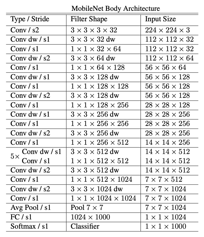
Mobilenet plug and play
Lets now use MobileNet as it is quite lightweight (17Mb), freeze the base layers and lets add and train the top few layers. Note only two classifiers.
# Use the mobilenet architecture as a starting point for our base model

# Import the mobilenet model with pre-trained imagenet weights
# Discard the last 1000 neuron layer ie. the final fully connected layer
base_model=MobileNet(___)
x=base_model.output

x=GlobalAveragePooling2D()(x)

# On top of mobile net, add a few dense layers with 'relu' activation

# Using functional API, add a dense layer with 1024 neurons
x=Dense(___)(x)

# Add a dense layer with 512 neurons
x=Dense(___)(x)

# Add a final layer with 2 neurons and softmax activation
preds=Dense(___)(x)
# Using the functional API of keras, specify the input from the base model and the output as `preds` described above

model=Model(___) #specify the inputs and outputs
### edTest(test_chow2) ###
# Submit an answer choice as a string below (eg. if you choose option C, put 'C')
answer2 = '___'
We will use pre-trained weights as the model has been trained already on the Imagenet dataset. We ensure all the weights are non-trainable. We will only train the last few dense layers.
### edTest(test_layers) ###
# For transfer learning, we need to freeze some layers. Below we freeze the first 10 layers

# Freeze the first 10 layers of the network to be non-trainable
for layer in model.layers[:10]:
    ___
Lets check the model architecture
### edTest(test_summary) ###
# Look at the summary of your model
model.___()
⏸ In the pre trained model from the exercise how many trainable params did you have?
(Please answer this in quiz)
### edTest(test_chow3) ###
# Submit an answer as 10,000 or 10000
answer3 = '___'
Now lets load the training data into the ImageDataGenerator. Specify path, and it automatically sends the data for training in batches, simplifying the code.
Compile the model. Now lets train it. Should take less than two minutes on a GTX1070 GPU.
Training the model
# We now train our model, but first we will compile it with an appropriate loss function and optimizer

# Adam optimizer
# loss function will be categorical crossentropy
# evaluation metric will be accuracy

model.compile(___)
# Fit the model using the step size for train and validation specified below
# Given the limited resources, please restrict the number of epochs to less than 5

step_size_train=train_generator.n//train_generator.batch_size
step_size_validation=validation_generator.n//validation_generator.batch_size

model.fit(___)
Model is now trained. Now lets test some independent input images to check the predictions.
Inference on unseen data
# A helper function that takes a standard image and converts it into a tensor that can be used by the model

def load_image(img_path, show=False):

    img = image.load_img(img_path, target_size=(224, 224))
    img_tensor = image.img_to_array(img)                    # (height, width, channels)
    img_tensor = np.expand_dims(img_tensor, axis=0)         # (1, height, width, channels), add a dimension because the model expects this shape: (batch_size, height, width, channels)
    img_tensor = preprocess_input(img_tensor)               # imshow expects values in the range [0, 1]

    if show:
        plt.imshow(img_tensor[0])
        plt.axis('off')
        plt.show()

    return img_tensor
# # We specify the paths of the six images

# We specify the paths of the six images
#31.jpg	458.jpg  571.jpg  667.jpg  672.jpg
# First set of images
img_path1 = os.path.join(DATA_DIR, 'resized_lecture18/test/31.jpg')
img_path2 = os.path.join(DATA_DIR, 'resized_lecture18/test/458.jpg')
img_path3 = os.path.join(DATA_DIR, 'resized_lecture18/test/571.jpg')


# Second set of images
img_path4 = os.path.join(DATA_DIR, 'resized_lecture18/test/rashmi.jpg')
img_path5 = os.path.join(DATA_DIR, 'resized_lecture18/test/pavlos.jpg')
img_path6 = os.path.join(DATA_DIR, 'resized_lecture18/test/shivas.jpg')
# Helper function that nicely predicts the class along with the input image

def prediction(img_loc,ax):
    new_image = load_image(img_loc)
    pred = model.predict(new_image)
    classmap = {v:k for k,v in (train_generator.class_indices).items()}
    plot_img = mpimg.imread(img_loc);
    ax.imshow(plot_img, vmin=0, vmax=255)
    ax.set_title(f'Prediction: {classmap[pred.argmax(-1)[0]]} \n (with confidence: {str(pred[0][pred.argmax(-1)][0])[:4]})'  ,fontsize=18)
    ax.axis('off')
# Make predictions on first set of images defined above that were never shown to the model before
fig, axes = plt.subplots(1,3,figsize=(12,6))

# For each prediction mention the axes
prediction(img_path1, axes[0])
prediction(img_path2, axes[1])
prediction(img_path3, axes[2])
# Make predictions on second set of images defined above that were never shown to the model before
fig, axes = plt.subplots(1,3,figsize=(15,5))

# # Call the prediction function defined above for this
# # For each prediction mention the axes
# ___
# ___
# ___

# For each prediction mention the axes
# For each prediction mention the axes
prediction(img_path4, axes[0])
prediction(img_path5, axes[1])
prediction(img_path6, axes[2])
Mindchow 🍲
Go back and change the number of trainable parameters. How does it affect your network performance?
Your answer here