Key Word(s): Convolutional Neural Network, Neural Networks, CNNs, MPL
Title :
Investigating CNNs
Description :
The goal of the exercise is to investigate the building blocks of a CNN, such as kernels, filters, and feature maps using a CNN model trained on the CIFAR-10 dataset.
Instructions:
- Import the CIFAR-10 dataset, and the pre-trained model from the helper file by calling the
get_cifar10()function. - Evaluate the model on the test set in order to verify if the selected model has trained weights. You should get a test set accuracy of about 75%.
- Take a quick look at the model architecture using
model.summary(). - Investigate the weights of the pre-trained model and plot the weights of the 1st filter of the 1st convolution layer.
- Plot all the filters of the first convolution layer.
- Use the helper code give to visualize the
feature mapsof the first convolution layer along with the input image. - Use the helper code give to visualize the
activationsof the first convolution layer along with the input image.
Hints:
model.layersAccesses various layers of the model
model.predict()Used to predict the values given the model
model.layers.get_weights()Get the weights of a particular layer
tensorflow.keras.Model()Functional API to group layers into an object with training and inference features.
Visual Demonstration of CNNs
# Import necessary libraries
import numpy as np
import random
import pandas as pd
import matplotlib.pyplot as plt
%matplotlib inline

import tensorflow as tf
from tensorflow.keras.models import Sequential, Model

from matplotlib import cm
import helper
from helper import cnn_model, get_cifar10, plot_featuremaps
# As we are using a pre-trained model,
# we will only use 1000 images from the 'unseen' test data
# The get_cifar10() function will load 1000 cifar10 images
(x_test, y_test) = get_cifar10()

# We also provide a handy dictionary to map response values to image labels
cifar10dict = helper.cifar10dict
cifar10dict
# Let's look at some sample images with their labels
# Run the helper code below to plot the image and its label
num_images = 5
fig, ax = plt.subplots(1,num_images,figsize=(12,12))
for i in range(num_images):
    image_index = random.randint(0,1000)
    img = (x_test[image_index] + 0.5)
    ax[i].imshow(img)
    label = cifar10dict[np.argmax(y_test[image_index])]
    ax[i].set_title(f'Actual: {label}')
    ax[i].axis('off')
# For this exercise we use a pre-trained network by calling
# the cnn_model() function
model = cnn_model()
model.summary()
# Evaluate the pretrained model on the test set
model_score = model.evaluate(x_test,y_test)
print(f'The test set accuracy for the pre-trained model is {100*model_score[1]:.2f} %')
# Visualizing the predictions on 5 randomly selected images
num_images = 5
fig, ax = plt.subplots(1,num_images,figsize=(12,12))
for i in range(num_images):
    image_index = random.randint(0,1000)
    prediction= cifar10dict[int(np.squeeze(np.argmax(model.predict(x_test[image_index:image_index+1]),axis=1),axis=0))]
    img = (x_test[image_index] + 0.5)
    ax[i].imshow(img)
    ax[i].set_title(f'Predicted: {prediction} \n Actual: {cifar10dict[np.argmax(y_test[image_index:image_index+1])]}')
    ax[i].axis('off')
Visualize kernels corresponding to the filters for the 1st layer
# The 'weights' variable is of the form
# [height, width, channel, number of filters]

# Use .get_weights() with the appropriate layer number
# to get the weights and bias of the first layer i.e. layer number 0
weights, bias= ___

assert weights.shape == (3,3,3,32), "Computed weights are incorrect"
# How many filters are in the first convolution layer?
n_filters = ___
print(f'Number of filters: {n_filters}')

# Print the filter size
filter_channel = ___
filter_height = ___
filter_width = ___
print(f'Number of channels {filter_channel}')
print(f'Filter height {filter_height}')
print(f'Filter width {filter_width}')
### edTest(test_chow1) ###
# Submit an answer choice as a string below (eg. if you choose option C, put 'C')
answer1 = '___'
# The 'weights' variable (defined above) is of the form
# [height, width, channel, number of filters]
# From this select all three channels, the entire length and width
# and the first filter
kernels_filter1 = ___

# Test case to check if you have indexed correctly
assert kernels_filter1.shape == (3,3,3)
# Use the helper code below to plot each kernel of the choosen filter
fig, axes = plt.subplots(1,3,figsize = (12,4))
colors = ['Reds','Greens','Blues']
for num, i in enumerate(axes):
  i.imshow(kernels_filter1[num],cmap=colors[num])
  i.set_title(f'Kernel for {colors[num]} channel')
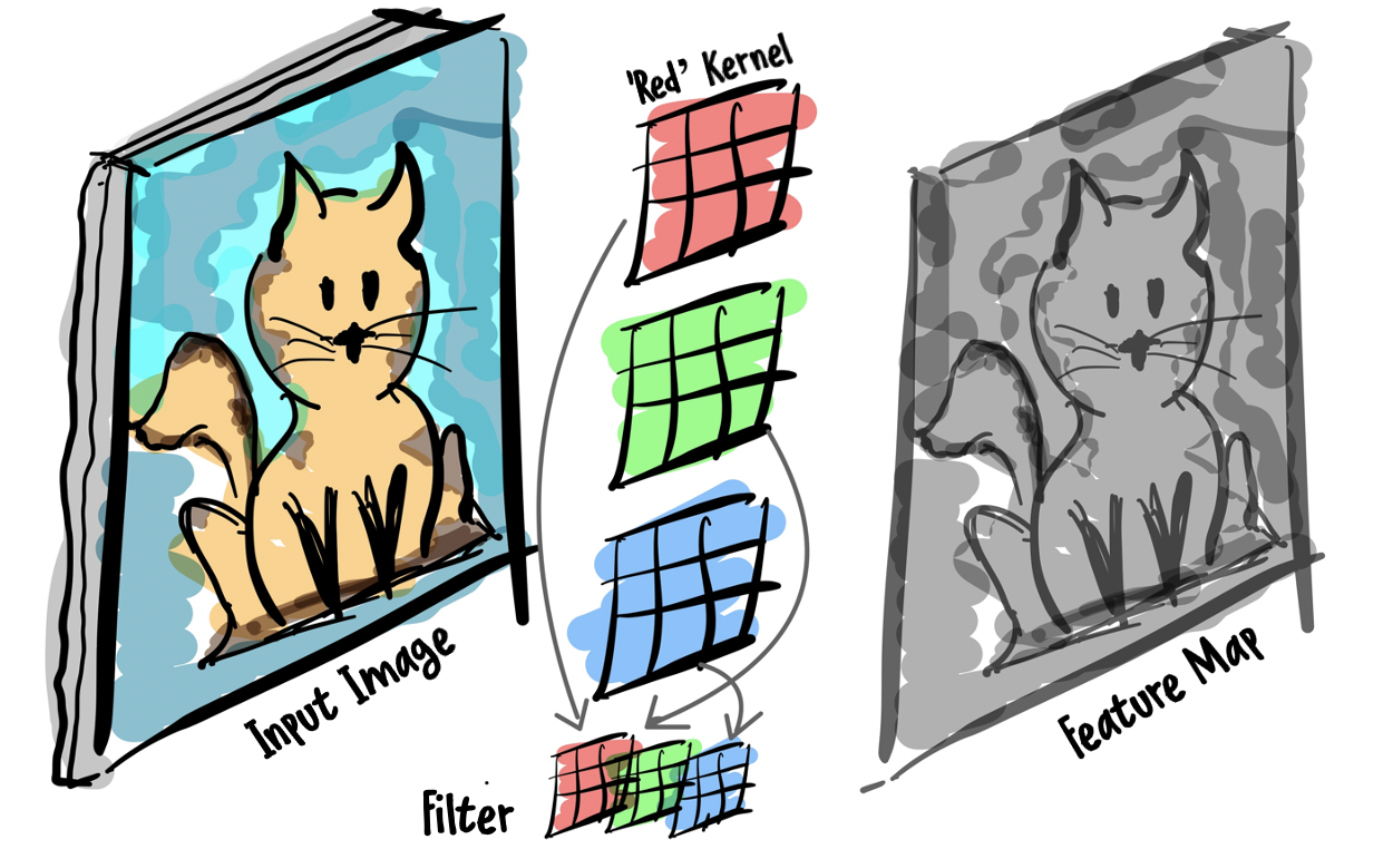
Visualizing one filter for the first convolutional layer
Each of the above kernels stacked together forms a filter, which interacts with the input.
# For the same filter above, we perform normalization because the current
# values are between -1 and 1 and the imshow function would truncate all values
# less than 0 making the visual difficult to infer from.
kernels_filter1 = (kernels_filter1 - kernels_filter1.min())/(kernels_filter1.max() - kernels_filter1.min())

# Plotting the filter
fig, ax = plt.subplots(1,1,figsize = (4,4))
ax.imshow(kernels_filter1)
ax.set_title(f'1st Filter of convolution')
Visualizing all the filters (32) for the first convolutional layer
# Use the helper code below to visualize all filters for the first layer

fig,ax=plt.subplots(4,8,figsize=(14,14))
fig.subplots_adjust(bottom=0.2,top=0.5)
for i in range(4):
    for j in range(8):
        filters= weights[:,:,:,(8*i)+j]
        filters = (filters - filters.min())/(filters.max() - filters.min())
        ax[i,j].imshow(filters)

fig.suptitle('All 32 filters for 1st convolution layer',fontsize=20, y=0.53);
Visualize Feature Maps & Activations
⏸ Which of the following statements is true?
A. Feature maps are a collection of weights, and filters are outputs of convolved inputs.
B. Filters are a collection of learned weights, and feature maps are outputs of convolved inputs.
C. Feature maps are learned features of a trained CNN model.
D. Filters are the outputs of an activation layer on a feature map.
### edTest(test_chow2) ###
# Submit an answer choice as a string below (eg. if you choose option C, put 'C')
answer2 = '___'
# Use model.layers to get a list of all the layers in the model
layers_list = ___
print('\n'.join([layer.name for layer in layers_list]))
For this exercise, we take a look at only the first convolution layer and the first activation layer.
# Get the output of the first convolution layer
layer0_output = model.layers[0].output
# Use the tf.keras functional API : Model(inputs= , outputs = ) where
# the input will come from model.input and output will be layer0_output
feature_model = ___

# Use a sample image from the test set to visualize the feature maps
img = x_test[16].reshape(1,32,32,3)

# NOTE: We have to reshape the image to 4-d tensor so that
# it can input to the trained model
# Use the helper code below to plot the feature maps
features = feature_model.predict(img)
plot_featuremaps(img,features,[model.layers[0].name])
Visualizing the first activation
# Get the output of the first activation layer
layer1_output = model.layers[1].output
# Follow the same steps as above for the next layer
activation_model = ___
# Use the helper code to again visualize the outputs
img = x_test[16].reshape(1,32,32,3)
activations = activation_model.predict(img)

# You can download the plot_featuremaps helper file
# to see how exactly do we make this nice plot below
plot_featuremaps(img,activations,[model.layers[1].name])
### edTest(test_chow3) ###
# Submit an answer choice as a string below
# (eg. if you choose option B, put 'B')
answer3 = '___'