import pandas as pd
import numpy as np
from matplotlib import pyplot as plt
from sklearn.decomposition import PCA
from sklearn.preprocessing import StandardScaler
%matplotlib inline

df = pd.read_csv('data2.csv')
display(df.describe())
df.head()

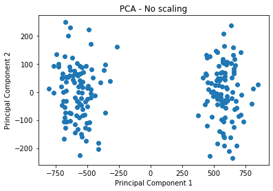
### edTest(test_pca_noscaling) ###
#Fit and Plot the first 2 principal components (no scaling)
fitted_pca = PCA().fit(____)
pca_result = fitted_pca.transform(____)
plt.scatter(pca_result[:,0],pca_result[:,1])
plt.xlabel("Principal Component 1")
plt.ylabel("Principal Component 2")
plt.title("PCA - No scaling");

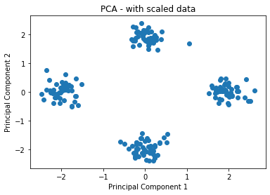
### edTest(test_pca_scaled) ###
#scale the data and plot first 2 principal components
scaled_df = StandardScaler().____
fitted_pca = PCA().fit(____)
pca_result = fitted_pca.transform(____)
plt.scatter(pca_result[:,0],pca_result[:,1])
plt.xlabel("Principal Component 1")
plt.ylabel("Principal Component 2")
plt.title("PCA - with scaled data");