Title : Ex: Polynomial Regression¶

Goal: Create cubic polynomial least-squares regression

Description¶

After fitting the model and getting the predictions, you should see the following plot:

Hints:¶

Formulas in statsmodels

sm.ols

numpy vander

Refer to lecture notebook.

Do not change any other code except the blanks.

In [1]:

import pandas as pd
import numpy as np
import matplotlib.pyplot as plt

import statsmodels.formula.api as sm

%matplotlib inline

In [2]:

df = pd.read_csv('data1.csv')
df = df.sort_values('x')
df.head()

Out[2]:

	x	y
73	0.006248	17.329551
142	0.104671	15.268703
34	0.246137	15.394678
17	0.420595	12.743181
5	0.455565	15.480800

In [3]:

plt.scatter(df.x, df.y);
plt.xlabel("x")
plt.ylabel("y")
plt.show()

Cubic polynomial least-squares regression of y on x¶

In [0]:

### edTest(test_ols_formula) ###
def fit_model(formula):
    return sm.ols(formula=formula, data=df).fit()

formula = _____ 
fit2_lm = fit_model(formula)

In [0]:

### edTest(test_predictions_summary) ###
#Get the predictions and the summary dataframe
poly_predictions = fit2_lm.______().___()
poly_predictions

In [0]:

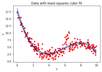
ax2 = df.plot.scatter(x='x',y='y',c='Red',title="Data with least-squares cubic fit")
ax2.set_xlabel("x")
ax2.set_ylabel("y")

# CI for the predection at each x value, i.e. the curve itself
ax2.plot(df.x, poly_predictions['mean'],color="green")
ax2.plot(df.x, poly_predictions['mean_ci_lower'], color="blue",linestyle="dashed")
ax2.plot(df.x, poly_predictions['mean_ci_upper'], color="blue",linestyle="dashed");

Condition number¶

In [0]:

c = np.vander(_, _, increasing=True)
np.linalg.cond(c)