Key Word(s): Gradient Descent, Stochastic Gradient Descent, Back Propagation, Optimizers
Instructions:
- Get the response and predictor variables from the backprop.csv file.
- Visualise the data generated.
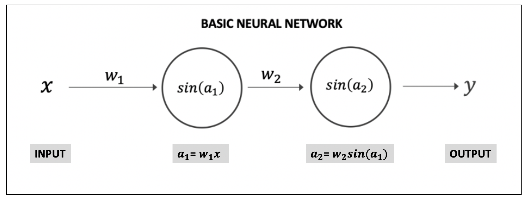
- For the given simple neural network, write a function that computes the gradient of the loss function with respect to the weights.
- To do this, compute the partial derivatives using individual functions. Refer to the instructions in the scaffold.
Hints:
The partial derivative of the loss function $L$ wrt $w_2$ and $w_1$ can be expressed as:
$$\frac{\partial L}{\partial w_2}\ =\ \frac{\partial L}{\partial y}\ \frac{\partial y}{\partial a_2}\frac{\partial a_2}{\partial w_2}$$$$\frac{\partial L}{\partial w_1}\ =\ \frac{\partial L}{\partial y}\ \frac{\partial y}{\partial a_2}\frac{\partial a_2}{\partial h_1}\ \frac{\partial h_1}{\partial a_1}\frac{\partial a_1}{\partial w_1}$$np.cos() : Returns cosine element-wise
np.sin() : Returns sine element-wise
v : Calculates the exponential of all elements in the input array.
NOTE - In this exercise, we expect you to take out a piece of paper an do the backpropagation using chain rule by hand.
In [1]:
# Import the necessary libraries

import pandas as pd
import matplotlib.pyplot as plt
%matplotlib inline
import numpy as np
In [48]:
# Read the file 'backprop.csv'

df = pd.read_csv('backprop.csv')
In [49]:
#Generating the predictor and response data
x = df.x.values.reshape(-1,1)
y = df.y.values
In [50]:
# Initialize the weights and use the same random seed as the previous exercise i.e. 310
np.random.seed(310)
W = [np.random.randn(1, 1), np.random.randn(1, 1)]
In [25]:
# Function to compute the activation function
def A(x):
    return ___

# Function to compute the derivative of the activation function
def der_A(x):
    return ___
In [47]:
# Defining a simple neural network we used in the previous exercise

def neural_network(W, x):

    # Computing the first affine
    a1 = np.dot(x, W[0])

    # Defining sin() as the activation function
    fa1 = A(a1)

    # Computing the second affine
    a2 = np.dot(fa1,W[1])

    # Defining sin() as the activation function
    y = A(a2)

    return a1,a2,y
In [51]:
#Use the helper code below to plot the true data and the predictions of your neural network

fig,ax = plt.subplots(1,1,figsize=(8,6))
ax.plot(x,y,label = 'True Function',color='darkblue',linewidth=2)
ax.plot(x,neural_network(W,x)[2],label = 'Neural Network Predictions',color='#9FC131FF',linewidth=2)
ax.set_xlabel('$x$',fontsize=14)
ax.set_ylabel('$y$',fontsize=14)
ax.legend(fontsize=14, loc='best');

In [26]:
# Function to compute the partial derivate of a (particular neuron) with respect to corresponding weight w

def dadw(x,firstweight=0):
    '''
    The derivative of the 'a' wrt the preceding weight is just the activation of the previous neuron
    Note, account for the case where the input layer has no activation layers associated with it. i.e return x if its the first weight
    '''
    if firstweight == 1:
        return ___
    return ___
In [27]:
# Function to compute the partial derivate of h with respect to a

def dhda(a):
    '''
    This is the derivative of the output of the activation function wrt the affine transformation.
    Return the derivative of the activation of the affine transformation
    '''

    return ___
In [ ]:
# Function to compute the partial derivate of y with respect to a

def dyda(a):
    '''
    This is the derivative of the output of the neural network wrt the affine transformation.
    Return the derivative of the activation of the affine transformation
    '''

    return ___
In [ ]:
# Function to compute the partial derivate of a with respect to h
def dadh(w):

    return ___
In [28]:
# Function to compute the partial derivate of loss with respect to y
def dldy(y_pred,y):
    '''
    Since our loss function is the MSE,
    The partial derivative of L wrt y will be 2*(y_pred - y), for all predictions and response
    '''

    return ___
In [46]:
# Function to compute the partial derivate of loss with respect to w

def dldw(W,x):

    '''
    Now, combine the functions from above and find the derivative wrt weights.
    These will be for all the points, hence take a mean of all values for each partial derivative and return as a list of 2 values

    '''
    dldw2 = ____
    dldw1 = ____

    return [np.mean(dldw2),np.mean(dldw1)]
In [52]:
### edTest(test_gradient) ###

# Get the predicted response, and the two activations of the network
a1, a2, y_pred = neural_network(W,x)

# Compute the gradient of the loss function with respect to the weights using function defined above
gradW = dldw(W,x)
In [ ]:
# Print the list of your gradients below
print(f'The derivatives of w1 w2 wrt L are {gradW}')
Mindchow 🍲
Compare your computed partial derivatives wrt the previous exercise. Are they the same?
This example was just for a simple case of 1 neuron in 1 hidden layer. How could we generalize this idea to compute partial derivatives of all the weights?