Title¶

Exercise: Back-propagation by hand

Description¶

The aim of this exercise is to perform back-propagation to update the weights of a simple neural network (shown below):

Instructions:¶

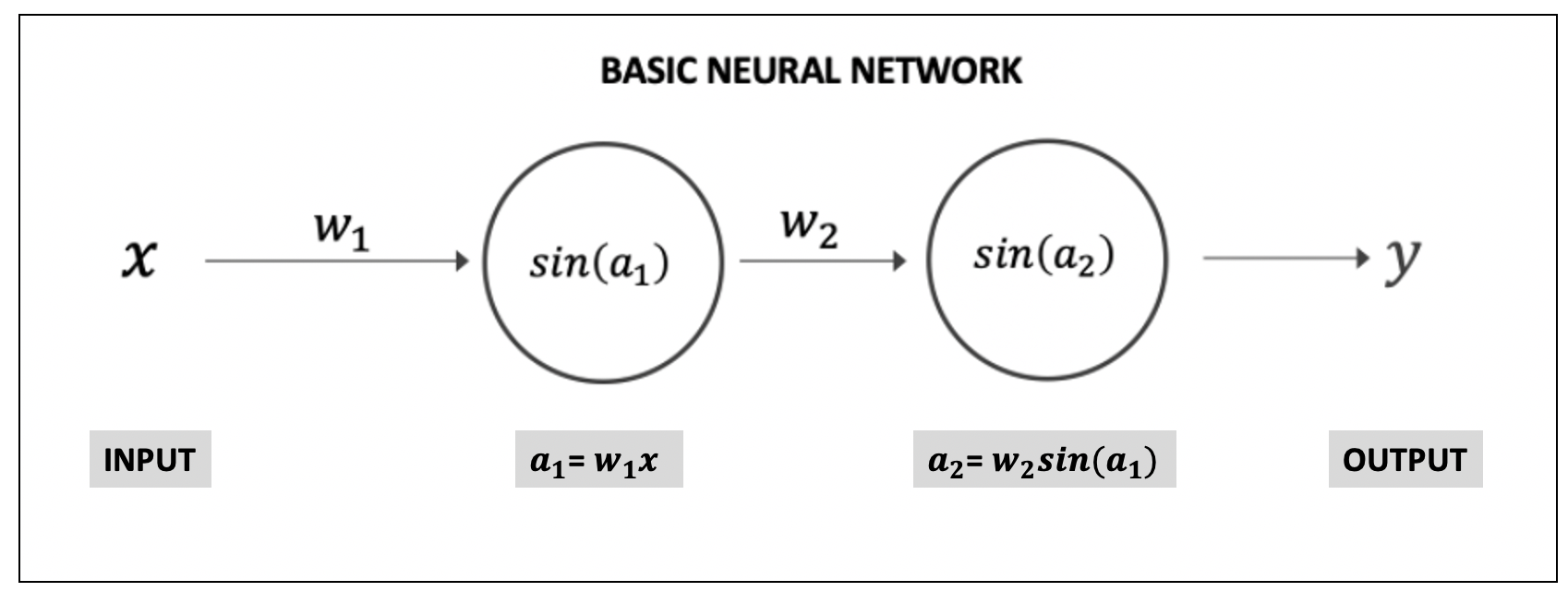
Get the predictor and response variables from the file backprop.csv and assign them to variables x and y.
Build a forward pass of the above neural network with one hidden layer. You will build this neural network using numpy (no deep learning package allowed).
Initialize the weights randomly with the random seed as 310, and make a prediction.
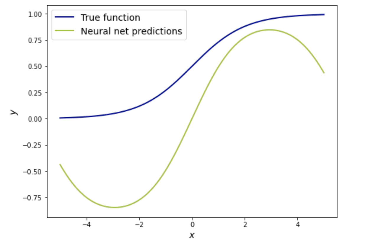
Plot your neural net predictions with the true value.

Compute the mean_squared_error of your predictions with the actual values.
Find the derivative of the loss function with respect to $w_1$.
Find the derivative of the loss function with respect to $w_2$.
Use the derivatives to update $w_1$ and $w_2$ .
Use the updated weights to make a forward pass and compute new predictions.
Plot the new predictions with the actual data. This will look similar to the one given above.
Calculate your $MSE$ and compare with the earlier value.

Hints:¶

Loss function:¶

$$L\ =\ \frac{1}{n}\sum_1^n\left(y_{pred}-y_{true}\right)^2$$

Activation function:¶

$$f\left(x\right)=\sin x$$

ax.plot() : A scatter plot of y vs. x with varying marker size and/or colour.

np.exp() : Calculates the exponential of all elements in the input array.

plt.xlabel() : This is used to specify the text to be displayed as the label for the x-axis.

plt.ylabel() : This is used to specify the text to be displayed as the label for the y-axis.

Note: This exercise is auto-graded and you can try multiple attempts.

In [1]:

# import required libraries

import pandas as pd
import numpy as np
import matplotlib.pyplot as plt
from sklearn.metrics import mean_squared_error
%matplotlib inline

In [2]:

# get the data from the file `backprop.csv`

df = pd.read_csv('backprop.csv')

# The input needs to be a 2D array so since we have a single
# column (1000,) we need to reshape to a 2D array (1000,1)

x = df.x.values.reshape(-1,1)

y = df.y.values

In [3]:

# Designing the simple neural network 

def neural_network(W, x):
    # W is a list of the two weights (w1,w2) of your neural network
    # x is the input to the neural network
    '''
    Compute a1, a2, and y
    a1 is the dot product of the input and weight
    To compute a2, first use the activation function on a1, then multiply by w2
    Finally, use the activation function on a2 to compute y
    Return all three values which you will use to compute derivatives later
    '''
    a1 = np.dot(___, ___)
    fa1 = np.sin(__)
    a2 = np.dot(___,___)
    y = np.sin(__)
    
    return a1,a2,y

In [4]:

# Initialize the weights, but keep the random seed as 310 for reproducable results

np.random.seed(310)
W = [np.random.randn(1, 1), np.random.randn(1, 1)]

In [ ]:

# Plot the predictor and response variables 

fig,ax = plt.subplots(1,1,figsize=(8,6))


# plot the true x and y values
ax.plot(x,y,label = 'True function',color='darkblue',linewidth=2)

# plot the x values with the network predictions

ax.plot(x,neural_network(W,x)[2],label = 'Neural net predictions',color='#9FC131FF',linewidth=2)

# Set the x and y labels
ax.set_xlabel('$x$',fontsize=14)
ax.set_ylabel('$y$',fontsize=14)
ax.legend(fontsize=14);

In [ ]:

### edTest(test_nn_mse) ###

# You can use the mean_squared_error function to find the MSE of your predictions with true function values
y_pred = ___
mse = mean_squared_error(y, y_pred)
print(f'The MSE of the neural network predictions wrt true function is {mse:.2f}')

Single update¶

In [5]:

# Here we will update the weights only once

# Get the predicted response, and the two a's of the network

a1,a2,y_pred = neural_network(W,x)

# Compute the gradient of the loss function with respect to weight 2
# Use pen and paper to calculate these derivatives before coding them

dldw2 = ___

# Now compute the gradient of the loss function with respect to weight 1

dldw1 = ___

# combine the two in a list
dldw = [np.mean(dldw1),np.mean(dldw2)]

---------------------------------------------------------------------------
NameError                                 Traceback (most recent call last)
 in 
      3 # Ge the predicted response, and the two activations of the network
      4 
----> 5 a1,a2,y_pred = neural_network(W,x)
      6 
      7 # Compute the gradient of the loss function with respect to weight 2

 in neural_network(W, x)
     13     ___
     14 
---> 15     return a1,a2,y

NameError: name 'a1' is not defined

In [ ]:

# In the update step, make sure to update the weights with their gradients

Wnew = [i - j for i,j in zip(W,dldw)]

In [ ]:

# Plot the predictor and response variables 

fig,ax = plt.subplots(1,1,figsize=(8,6))
ax.plot(x,y,label = 'True function',color='darkblue',linewidth=2)
ax.plot(x,neural_network(Wnew,x)[2],label = 'Neural net predictions',color='#9FC131FF',linewidth=2)
ax.set_xlabel('$x$',fontsize=14)
ax.set_ylabel('$y$',fontsize=14)
ax.legend(fontsize=14);

In [ ]:

### edTest(test_one_update_mse) ###
# Compute the new MSE after one update and print it
y_pred = ___
mse_update = ___
print(f'The MSE of the new neural network predictions with true function is {mse_update:.2f} as compared to {mse:.2f} from before ')

Several updates¶

In principle, only a single update will never be sufficient to improve model predictions. In the below segment, use the method from above, and update the weight 300 times before plotting predictions.

Does your MSE decrease?

In [ ]:

# Reinitialize the weights to start again 
np.random.seed(310)
W = [np.random.randn(1, 1), np.random.randn(1, 1)]

In [ ]:

# Unlike the previous step, this time we will set a learning rate of 0.01 to avoid drastic updates and run the above code for 10000 loops

lmb = 0.01
for i in range(300):
    a1,a2,y_pred = ___

    # Remember to use np.mean
    dldw2 = ___
    dldw1 = ___
    
    W[0] = W[0] - lmb * dldw1
    W[1] = W[1] - lmb * dldw2

In [ ]:

# Plot your results and calculate the MSE 

# Plot the predictor and response variables 
fig,ax = plt.subplots(1,1,figsize=(8,6))
ax.plot(x,y,label = 'True function',color='darkblue',linewidth=2)
ax.plot(x,neural_network(W,x)[2],label = 'Neural net predictions',color='#9FC131FF',linewidth=2)
ax.set_xlabel('$x$',fontsize=14)
ax.set_ylabel('$y$',fontsize=14)
ax.legend(fontsize=14);

In [ ]:

### edTest(test_mse) ###
# We again compute the MSE and compare it with the original predictions
y_pred = ___
mse_final = mean_squared_error(y,y_pred)
print(f'The final MSE is {mse_final:.2f} as compared to {mse:.2f} from before ')

Mindchow 🍲¶

If you notice, your predicted values are off by approximately 0.5, from the actual values. After marking, go back to your neural network and add a bias correction to your predictions of 0.5. i.e y = np.sin(a2) + 0.5 and rerun your code.

Does your code fit better? And does your $MSE$ reduce?

In [ ]: