Key Word(s): Neural Networks, Gradient Descent
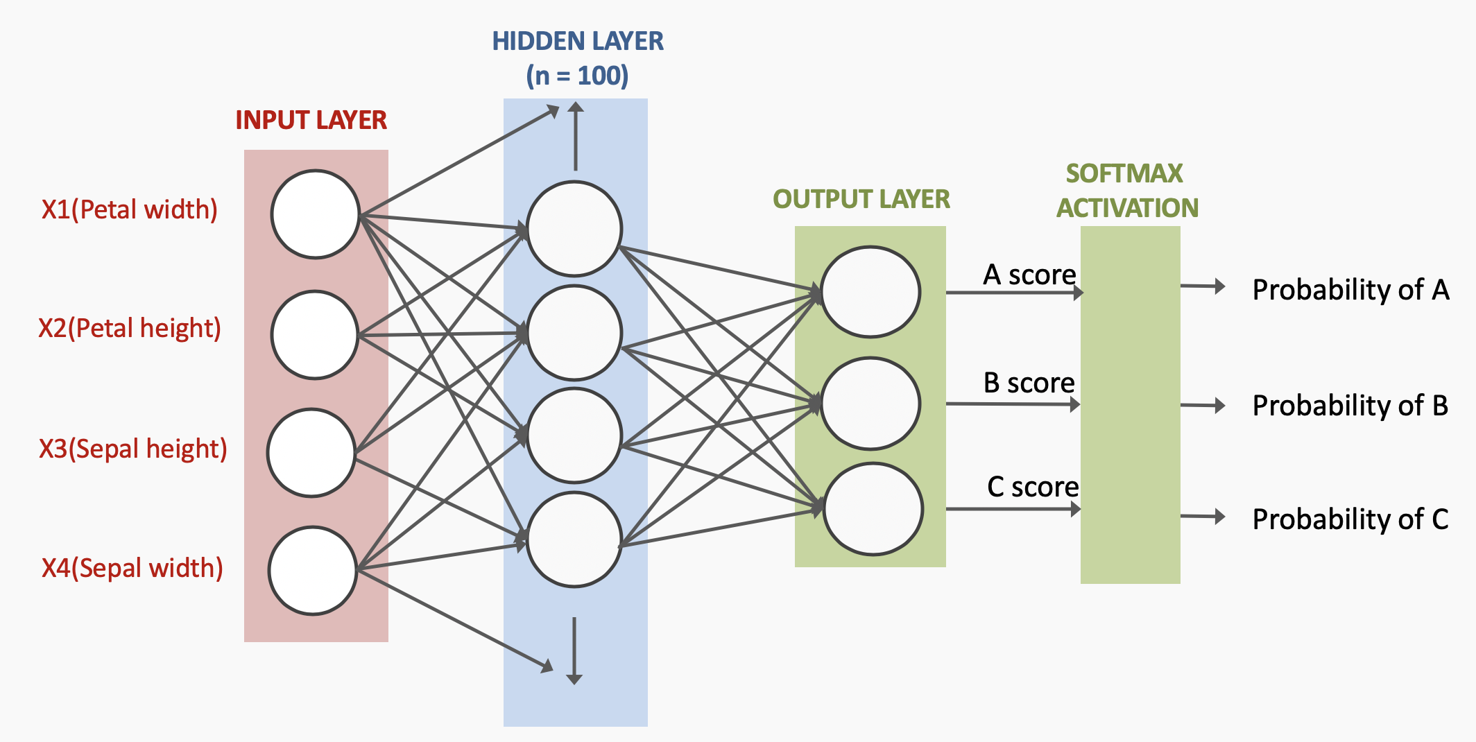
The dataset used here is the Iris dataset, same as the one used for logistic regression classification. This dataset has several features such as sepal length, sepal width and so on, to predict which of the iris species that particular flower belongs to here.
Instructions:
- Read the csv file as a pandas dataframe.
- Assign the dependent and independent variables. The species is your dependent variable. All the other columns are your predictors.
- Split the dataset into train and validation sets.
- Define the network parameters for the MLP.
- Initialise the weights and biases of the network.
- Define the MLP model with input, hidden and output layers.
- Fit the model on the training data.
- Compute and print the train and validation accuracy.
- Compare the output of the MLP classifier with that of the logistic model you had earlier fit in
Session 5 Exercise B.1. Find out which model performs better and why it does so?
Hints:
keras.add() : To add a layer to the model
keras.fit() : Fit the model for the data
model.evaluate() : Evaluate model performance on predictors vs true values
Note: This exercise is auto-graded and you can try multiple attempts.
In [ ]:
# Import the necessary libraries
import tensorflow as tf
import numpy as np
import matplotlib.pyplot as plt
from sklearn.model_selection import train_test_split
import pandas as pd
%matplotlib inline

tf.keras.backend.clear_session()  # For easy reset of notebook state.
In [ ]:
# Read the file 'IRIS.csv'

df = pd.read_csv('IRIS.csv')
In [ ]:
# Take a quick look at the dataset
df.head()
In [ ]:
# We use one-hot-encoding to encode the 'species' labels using pd.get_dummies

one_hot_df = pd.get_dummies(df[___], prefix='species')
In [ ]:
# The predictor variables are all columns except species
X = df.drop([___],axis=1).values

# The response variable is the one-hot-encoded species values
y = one_hot_df.values
In [ ]:
# We divide our data into test and train sets with 80% training size

X_train, X_test, y_train, y_test = train_test_split(___,___,train_size=___)
In [ ]:
# To build the MLP, we will use the keras library

model = tf.keras.models.Sequential(name='MLP')

# To initialise our model we set some parameters
# commonly defined in an MLP design

# The number of nodes in a hidden layer
n_hidden = ___

# The number of nodes in the input layer (features)
n_input = ___

# The number of nodes in the output layer
n_output = ___
In [ ]:
# We add the first hidden layer with `n_hidden` number of neurons
# and 'relu' activation
model.add((tf.keras.layers.Dense(n_hidden,input_dim=___, activation = ___,name='hidden')))

# The second layer is the final layer in our case, using 'softmax' on the output labels
model.add(tf.keras.layers.Dense(n_output, activation = ___,name='output'))
In [ ]:
# Now we compile the model using 'categorical_crossentropy' loss,
# optimizer as 'sgd' and 'accuracy' as a metric
model.compile(optimizer=___,
              loss=___,
              metrics=[___])
In [ ]:
# You can see an overview of the model you built using .summary()
model.summary()
In [ ]:
# We fit the model, and save it to a variable 'history' that can be
# accessed later to analyze the training profile
# We also set validation_split=0.2 for 20% of training data to be
# used for validation
# verbose=0 means you will not see the output after every epoch.
# Set verbose=1 to see it

history = model.fit(___,___, epochs = ___, batch_size = 16,verbose=0,validation_split=___)
In [ ]:
# Here we plot the training and validation loss and accuracy

fig, ax = plt.subplots(1,2,figsize = (16,4))
ax[0].plot(history.history['loss'],'r',label = 'Training Loss')
ax[0].plot(history.history['val_loss'],'b',label = 'Validation Loss')
ax[1].plot(history.history['accuracy'],'r',label = 'Training Accuracy')
ax[1].plot(history.history['val_accuracy'],'b',label = 'Validation Accuracy')
ax[0].legend()
ax[1].legend()
ax[0].set_xlabel('Epochs')
ax[1].set_xlabel('Epochs');
ax[0].set_ylabel('Loss')
ax[1].set_ylabel('Accuracy %');
fig.suptitle('MLP Training', fontsize = 24)
In [ ]:
### edTest(test_accuracy) ###
# Once you have near-perfect validation accuracy, time to evaluate model performance on test set

train_accuracy = model.evaluate(___,___)[1]
test_accuracy = model.evaluate(___,___)[1]
print(f'The training set accuracy for the model is {train_accuracy}\
    \n The test set accuracy for the model is {test_accuracy}')