Key Word(s): Neural Networks
Title
Exercise A.1 - Constructing an MLP
Description
From the exercise A.1, we observe that a single neuron is rather limited in what it can accomplish. But what if we expand the number of neurons in our network to make it more expressive?
The aim of this exercise is to construct an MLP learn its parameters from data using the Keras API which is part of Tensorflow 2.x.
TensorFlow is a framework for representing complicated DNN algorithms and executing them in any platform, from a phone to a distributed system using GPUs. Developed by Google Brain, TensorFlow is used very widely today.
Keras is a high-level API used for fast prototyping, advanced research, and production. We will use tf.keras which is TensorFlow's implementation of the Keras API.
You can learn more about Keras here.
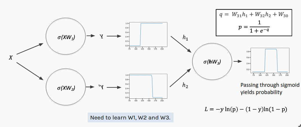 [Note: In this image $W$ matrices include both weight and bias terms and the vector input $x$ has been augmented into the matrix $X$ by adding a column of ones]
- In our example, we have a single input, $x$
- The first layer consists of 2 nodes (or neurons), each with its own weight and bias used to perform an affine transformation on the nodes' respective inputs. We refer to this as the 'hidden' layer.
- Both nodes in the hidden layer use the same activation function of the form $\sigma\left(\cdot\right)$ on their affine transformations.
- The outputs of the hidden layer nodes must then be combined to give the overall output of the network. This is the output layer. Because we will interpret the output as a probability we just take a linear combination of the hidden layer and pass it through another sigmoid activation to produce the actual prediction, $y$. Notice that the output layer has its own weights and bias.
This multilayer perceptron is much more expressive than a single perceptron, but setting all the new parameters manually would be quite tedious. And in larger networks, it's completely infeasible!
Instructions:
- Read the heart dataset as a pandas dataframe
- Assign the predictor and response variable and plot the data.
- Instantiate a Keras model
- Add a hidden layer with 2 nodes and a sigmoid activation function
- Add an output layer by choosing the number of nodes and the activation function
- Compile the model with binary cross-entropy as the loss function
- Fit the data on the model by specifying the number of epochs.
- Plot the training history
- Predict using the model and compute the accuracy
Hints:
keras.add() : To add a layer to the model
keras.fit() : Fit the model for the data
Note: This exercise is auto-graded and you can try multiple attempts.
#Import libraries
import numpy as np
import pandas as pd
import matplotlib.pyplot as plt

import tensorflow as tf
from tensorflow import keras
from tensorflow.keras import layers
from tensorflow.keras import models
%matplotlib inline
# We set a random seed to ensure our results are reproducible
seed = 399
np.random.seed(seed)
tf.random.set_seed(seed)
Multilayer Perceptron
We're using a slightly altered version of heart data from the previous exercise to illustrate a concept. Notice how now a single sigmoid will not be able to do an acceptible job of classification.
#Read the data and assign predictor and reponse variables
altered_heart_data = pd.read_csv('data/altered_heart_data.csv')
x = altered_heart_data.MaxHR.values
y = altered_heart_data.AHD.values
#Plot the data
plt.scatter(x, y, alpha=0.2)
plt.xlabel('MaxHR')
plt.ylabel('Heart Disease (AHD)');
Now we will use Keras to construct our MLP. You only need to add the output layer. Each step is described in the comments.
## First we instantiate a Keras model
MLP = models.Sequential(name='MLP')

## [Adding Layers]
# Next we add a hidden layer with 2 nodes and a sigmoid activation function
MLP.add(layers.Dense(2, activation='sigmoid', input_shape=(1,), name='hidden'))

# Now add the output layer
# Use the code above as an example. You only need to change the arguments
# Choose number of nodes and activation and name it 'output'
# (the input shape will be infered from the hidden layer's output shape)
# your code here
________

# [Compilation]
# here we set the loss to be minimized and a metric to monitor when fitting the MLP
MLP.compile(loss='binary_crossentropy', metrics=['accuracy'])
This simple model benefits from setting some reasonable initial weights. During fitting these weights will be optimized.
# Get original random weights
weights = MLP.get_weights()

# Hidden layer
# Weights
weights[0][0]=np.array([ 3.1,-3.2])

# Biases
weights[1]=np.array([-350.,402.])


# Output layer
# Weights
weights[2]=np.array([[1.29],[1.11]])

# Biases
weights[3] = np.array([-1.11])

# Update weights
MLP.set_weights(weights)
You should always inspect your Keras model with the summary() method. Note the number of parameters in each layer:
Hidden has 4 - it contains 2 nodes each with a weight and bias.
Output has 3 - it has a weight for each node in the previous layer plus a bias term.
#View model summary
MLP.summary()
Now we fit (or 'train') the MLP on our data, updating the weights to minimize the loss we specified in the call to compile(). (There will be more details on how this update happens in future lectures).
One full training cycle on our data is called an 'epoch.' Usually multiple epochs are required before a model converges. Specify a number of epochs to train for.
#Fit the model on the data by specifing number of epochs
MLP.fit(___);
We can plot the training history and observe that as the weights were updated our loss declined and the accuracy improved.
#Plotting the model history
history = MLP.history.history
fig, ax = plt.subplots(1,2, figsize=(10,4))
ax[0].plot(history['loss'], c='r', label='loss')
ax[0].set_ylabel('crossentropy loss')
ax[1].plot(history['accuracy'], c='b')
ax[1].set_ylabel('accuracy')
for axis in ax:
    axis.set_xlabel('epoch')
Let's look at the individual outputs of the 2 nodes in the hidden layer.
# Create xs for input to predict on
x_linspace = np.linspace(np.min(x), np.max(x), 500)

# Get output from the hidden layer nodes
hidden = models.Model(inputs=MLP.input, outputs=MLP.get_layer('hidden').output)
hidden_pred = hidden.predict(x_linspace)

h1_pred = hidden_pred[:,0]
h2_pred = hidden_pred[:,1]
#Plot output from h1 & h2
fig, ax = plt.subplots(1,1, figsize=(14,10))
ax.scatter(x, y, alpha=0.4, label='Altered Heart Data')
ax.plot(x_linspace, h1_pred, lw=4, alpha=0.6, label=r'$h_1 = \sigma(W_1x+\beta_1)$')
ax.plot(x_linspace, h2_pred, lw=4, alpha=0.6, label=r'$h_2 = \sigma(W_2x+\beta_2)$')

# Set title
ax.set_title('Hidden Layer Nodes', fontsize=24)

# Create labels (very important!)
ax.set_xlabel('$x$', fontsize=24) # Notice we make the labels big enough to read
ax.set_ylabel('$y$', fontsize=24)

ax.tick_params(labelsize=24) # Make the tick labels big enough to read

ax.legend(fontsize=24, loc='best'); # Create a legend and make it big enough to read
We can see that each node in the hidden layer indeed outputs a different sigmoid.
Now let's look at how they are combined by the output layer.
# Get output layer predictions
y_pred = MLP.predict(x_linspace)
# Plot predictions
fig, ax = plt.subplots(1,1, figsize=(14,10))

ax.scatter(x, y, alpha=0.4, label=r'Altered Heart Data')
ax.plot(x_linspace, y_pred, lw=4, label=r'$y_{pred} = \sigma(W_3h_{1} + W_4h_{2}+\beta_{3})$')

# Create labels (very important!)
ax.set_xlabel('$x$', fontsize=24) # Notice we make the labels big enough to read
ax.set_ylabel('$y$', fontsize=24)

ax.tick_params(labelsize=24) # Make the tick labels big enough to read

ax.legend(fontsize=24, loc='best'); # Create a legend and make it big enough to read
Finally, let's compare the MLP's accuracy to a baseline that always predicts the majority class. Try and see if you can get over 80% accuracy (86%+ is possible). You may need to change the number of epochs above and rerun the notebook.
def accuracy(y_true, y_pred):
    assert y_true.shape[0] == y_pred.shape[0]
    return sum(y_true == (y_pred >= 0.5).astype(int))/len(y_true)
### edTest(test_performance) ###
final_pred = MLP.predict(x).flatten()

baseline_acc = accuracy(y, np.zeros(len(y))) # predictions are all zeros
MLP_acc = accuracy(y, final_pred)
print(f'Baseline Accuracy: {baseline_acc:.2%}')
print(f'MLP Accuracy: {MLP_acc:.2%}')