Key Word(s): Neural Networks, Perceptron, MLP
Instructions:
The Neural Network will be built from scratch using pre-trained weights and biases. Hence, we will only be doing the forward (i.e., prediction) pass.
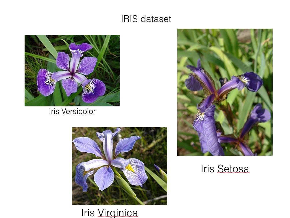
- Load the iris dataset from sklearn standard datasets.
- Assign the predictor and response variables appropriately.
- One hot encode the categorical labels of the predictor variable.
- Load and inspect the pre-trained weights and biases.
- Construct the MLP:
- Augment X with a column of ones to create the augmented design matrix X
- Create the first layer weight matrix by vertically stacking the bias vector on top of the weight vector
- Perform the affine transformation
- Activate the output of the affine transformation using ReLU
- Repeat the first 3 steps for the hidden layer (augment, vertical stack, affine)
- Use softmax on the final layer
- Finally, predict y
Hints:
This will further develop our intuition for the architecture of a deep neural network. This diagram shows the structure of our network. You may find it useful to refer to it during the exercise.
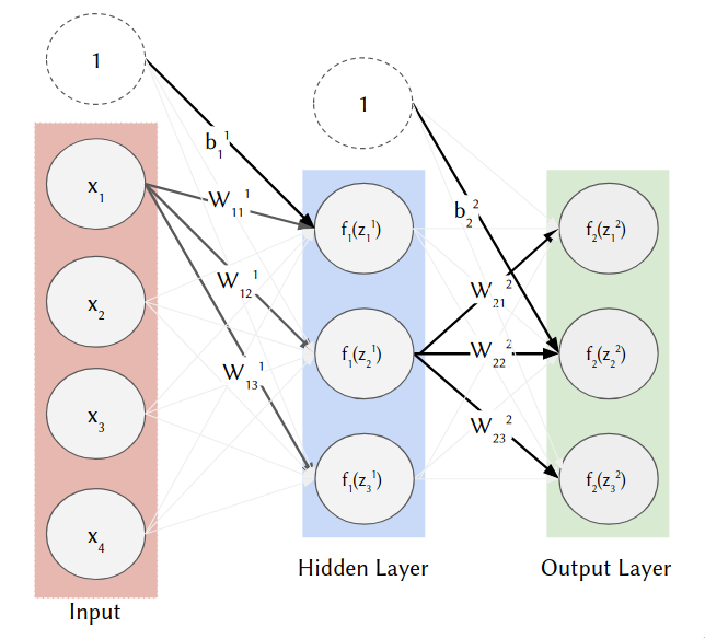
This is our first encounter with a multi-class classification problem and also the softmax activation on the output layer. Note: $f_1()$ above is the ReLU activation and $f_2()$ is the softmax.
to_categorical(y, num_classes=None, dtype='float32') : Converts a class vector (integers) to the binary class matrix.
np.vstack(tup) : Stack arrays in sequence vertically (row-wise).
numpy.dot(a, b, out=None) : Returns the dot product of two arrays.
numpy.argmax(a, axis=None, out=None) : Returns the indices of the maximum values along an axis.
Note: This exercise is auto-graded and you can try multiple attempts.
#Import library
import numpy as np
import matplotlib.pyplot as plt
import tensorflow as tf
from sklearn.datasets import load_iris
from tensorflow.keras.utils import to_categorical
%matplotlib inline
#Load the iris data
iris_data = load_iris()

#Get the predictor and reponse variables
X = iris_data.data
y = iris_data.target

#See the shape of the data
print(f'X shape: {X.shape}')
print(f'y shape: {y.shape}')
#One-hot encode target labels
Y = to_categorical(y)
print(f'Y shape: {Y.shape}')
Load and inspect the pre-trained weights and biases. Compare their shapes to the NN diagram.
#Load and inspect the pre-trained weights and biases
weights = np.load('data/weights.npy', allow_pickle=True)

# weights for hidden (1st) layer
w1 = weights[0]

# biases for hidden (1st) layer
b1 = weights[1]

# weights for output (2nd) layer
w2 = weights[2]

#biases for output (2nd) layer
b2 = weights[3]
#Compare their shapes to that in the NN diagram.
for arr, name in zip([w1,b1,w2,b2], ['w1','b1','w2','b2']):
    print(f'{name} - shape: {arr.shape}')
    print(arr)
    print()
For the first affine transformation we need to multiple the augmented input by the first weight matrix (i.e., layer).
$$ \begin{bmatrix} 1 & X_{11} & X_{12} & X_{13} & X_{14}\\ 1 & X_{21} & X_{22} & X_{23} & X_{24}\\ \vdots & \vdots & \vdots & \vdots & \vdots \\ 1 & X_{n1} & X_{n2} & X_{n3} & X_{n4}\\ \end{bmatrix} \begin{bmatrix} b_{1}^1 & b_{2}^1 & b_{3}^1\\ W_{11}^1 & W_{12}^1 & W_{13}^1\\ W_{21}^1 & W_{22}^1 & W_{23}^1\\ W_{31}^1 & W_{32}^1 & W_{33}^1\\ W_{41}^1 & W_{42}^1 & W_{43}^1\\ \end{bmatrix} = \begin{bmatrix} z_{11}^1 & z_{12}^1 & z_{13}^1\\ z_{21}^1 & z_{22}^1 & z_{23}^1\\ \vdots & \vdots & \vdots \\ z_{n1}^1 & z_{n2}^1 & z_{n3}^1\\ \end{bmatrix} = \textbf{Z}^{(1)} $$About the notation: superscript refers to the layer and subscript refers to the index in the particular matrix. So $W_{23}^1$ is the weight in the 1st layer connecting the 2nd input to 3rd hidden node. Compare this matrix representation to the slide image. Also note the bias terms and ones that have been added to 'augment' certain matrices. You could consider $b_1^1$ to be $W_{01}^1$.
1. Augment X with a column of ones to create `X_aug`2. Create the first layer weight matrix `W1` by vertically stacking the bias vector `b1`on top of `w1` (consult `add_ones_col` for ideas. Don't forget your `Tab` and `Shift+Tab` tricks!)3. Do the matrix multiplication to find `Z1`def add_ones_col(X):
'''Augment matrix with a column of ones'''
X_aug = np.hstack((np.ones((X.shape[0],1)), X))
return X_aug
#Use add_ones_col()
X_aug = add_ones_col(___)

#Use np.vstack to add biases to weight matrix
W1 = np.vstack((___,___))

#Use np.dot() to multiple X_aug and W1
Z1 = np.dot(___,___)
Next, we use our non-linearity $$ \textit{a}_{\text{relu}}(\textbf{Z}^{(1)})= \begin{bmatrix} h_{11} & h_{12} & h_{13}\\ h_{21} & h_{22} & h_{23}\\ \vdots & \vdots & \vdots \\ h_{n1} & h_{n2} & h_{n3}\\ \end{bmatrix}= \textbf{H} $$
1. Define the ReLU activation
2. use `plot_activation_func` to confirm implementation 3. Use relu on `Z1` to create `H`def relu(z: np.array) -> np.array:
# hint:
# relu(z) = 0 when z < 0
# otherwise relu(z) = z
# your code here
h = np.maximum(___,___) # np.maximum() will help
return h
#Helper code to plot the activation function
def plot_activation_func(f, name):
    lin_x = np.linspace(-10,10,200)
    h = f(lin_x)
    plt.plot(lin_x, h)
    plt.xlabel('x')
    plt.ylabel('y')
    plt.title(f'{name} Activation Function')

plot_activation_func(relu, name='RELU')
# use your relu activation function on Z1
H = relu(___)
The next step is very similar to the first and so we've filled it in for you.
$$ \begin{bmatrix} 1 & h_{11} & h_{12} & h_{13}\\ 1 & h_{21} & h_{22} & h_{23}\\ \vdots & \vdots & \vdots & \vdots \\ 1 & h_{n1} & h_{n2} & h_{n3}\\ \end{bmatrix} \begin{bmatrix} b_{1}^{(2)} & b_{2}^2 & b_{3}^2\\ W_{11}^2 & W_{12}^2 & W_{13}^2\\ W_{21}^2 & W_{22}^2 & W_{23}^2\\ W_{31}^2 & W_{32}^2 & W_{33}^2\\ \end{bmatrix}= \begin{bmatrix} z_{11}^2 & z_{12}^2 & z_{13}^2\\ z_{21}^2 & z_{22}^2 & z_{23}^2\\ \vdots & \vdots & \vdots \\ z_{n1}^2 & z_{n2}^2 & z_{n3}^2\\ \end{bmatrix} = \textbf{Z}^{(2)} $$1. Augment `H` with ones to create `H_aug`
2. Combine `w2` and `b2` to create the output weight matric `W2` 3. Perform the matrix multiplication to produce `Z2`#Use add_ones_col()
H_aug = ___
#Use np.vstack to add biases to weight matrix
W2 = ___
#Use np.dot()
Z2 = np.dot(H_aug,W2)
Finally we use the softmax activation on Z2. Now for each observation we have an output vector of length 3 which can be interpreted as a probability (they sum to 1).
$$
\textit{a}_{\text{softmax}}(\textbf{Z}^2)=
\begin{bmatrix}
\hat{y}_{11} & \hat{y}_{12} & \hat{y}_{13}\\
\hat{y}_{21} & \hat{y}_{22} & \hat{y}_{23}\\
\vdots & \vdots & \vdots \\
\hat{y}_{n1} & \hat{y}_{n2} & \hat{y}_{n3}\\
\end{bmatrix}
= \hat{\textbf{Y}}
$$
1. Define softmax
2. Use `softmax` on `Z2` to create `Y_hat`def softmax(z: np.array) -> np.array:
'''
Input: z - 2D numpy array of logits
rows are observations, classes are columns
Returns: y_hat - 2D numpy array of probabilities
rows are observations, classes are columns
'''
# hint: we are summing across the columns
y_hat = np.exp(___)/np.sum(np.exp(___), axis=___, keepdims=True)
return y_hat
#Calling the softmax function
Y_hat = softmax(___)
Now let's see how accuract the model's predictions are! Use `np.argmax` to collapse the columns of `Y_hat` to create `y_hat`, a vector of class labels like the original `y` before one-hot encoding.
### edTest(test_acc) ###

# Compute the accuracy
y_hat = np.argmax(___, axis=___)
acc = sum(y == y_hat)/len(y)
print(f'accuracy: {acc:.2%}')