Key Word(s): bagging
Instructions:
- Read the dataset
agriland.csv. - Assign the predictor and response variables as
Xandy. - Split the data into train and test sets with
test_split=0.2andrandom_state=44. - Fit a single
DecisionTreeClassifier()and find the accuracy of your prediction. - Complete the helper function
prediction_by_bagging()to find the average predictions for a given number of bootstraps. - Now perform Bagging using the helper function, and compute the new accuracy.
- Proceed to plot of accuracy with increasing number of bootstraps.
- Finally, use the helper code to plot the decision boundaries for varying
max_depthalong withnum_bootstraps. Investigate the effect of increasing bootstraps on the variance.
Hints:
sklearn.tree.DecisionTreeClassifier() : A decision tree classifier.
np.random.choice : Generates a random sample from a given 1-D array
plt.subplots() : Create a figure and a set of subplots.
ax.plot() : Plot y versus x as lines and/or markers
Note: This exercise is auto-graded and you can try multiple attempts.
Bagging Classification
# Import required libraries

%matplotlib inline
import pandas as pd
import numpy as np
import matplotlib.pyplot as plt
from sklearn.tree import DecisionTreeClassifier
from sklearn.model_selection import train_test_split
from sklearn import metrics
import scipy.optimize as opt
from sklearn.metrics import accuracy_score

# to be used for plotting later

from matplotlib.colors import ListedColormap
cmap_light = ListedColormap(['#FFF4E5','#D2E3EF'])
cmap_bold = ListedColormap(['#F7345E','#80C3BD'])
# Read the file 'agriland.csv' and take a quick look at your data
df = pd.read_csv('agriland.csv')

# Note that the latitude & longitude values are normalized
df.head()
# Set your predictor variables(latitude &longitude;) as 'X' and response variable as y and make sure to use .values

X = ___

y = ___
#split data in train an test, with test size = 0.2 and randomstate=44

X_train, X_test, y_train, y_test = train_test_split(X, y, test_size=0.2,random_state=44)
# Define the max_depth of your decision tree and set the random_state variable as 44

max_depth = ___

# Lets create and train our model
clf = DecisionTreeClassifier(max_depth=max_depth, random_state=44)

clf.fit(X_train, y_train)
# Predict on the test set and calculate the accuracy of a single decision tree

prediction = ___
single_acc = ___
print(f'Single tree Accuracy is {single_acc*100}%')
# Complete the function below to get the prediction by bagging

# Inputs: X_train, y_train to train your data
# X_to_evaluate: Samples that you are goin to predict (evaluate)
# num_bootstraps: how many trees you want to train
# Output: An array of predicted classes for X_to_evaluate

def prediction_by_bagging(X_train, y_train, X_to_evaluate, num_bootstraps):

    # list to store every array of predictions

    predictions = []

    #generate num_bootstraps number of trees

    for i in range(num_bootstraps):

        # sample data to perform first bootstrap, here, we actually bootstrap indices, because we want the same subset for X_train and y_train

        resample_indexes = np.random.choice(np.arange(y_train.shape[0]), size=y_train.shape[0])

        # get bootstrapped set for 'X' and 'y' using the above indices

        X_boot = X_train[___]
        y_boot = y_train[___]

        # train decision tree on bootstrap set, use the same max_depth and random_state as above

        clf = ___

        # fit the model on bootstrapped training set

        clf.fit(___,___)

        #  make predictions on X_to_evaluate samples

        pred = clf.predict(___)

        predictions.append(pred)
    # Now we have a list of predictions like [prediction_array_0, prediction_array_1, ..., prediction_array_n]

    # To get the majority vote for each sample, we can find the average prediction and threshold them by 0.5

    average_prediction = ___

    return average_prediction
### edTest(test_bag_acc) ###
# now we print the accuracy of the bagging with decision trees

#Define the number of bootstraps to be used

num_bootstraps = 200

y_pred = prediction_by_bagging(X_train,y_train,X_test,num_bootstraps=num_bootstraps)

# Compare the average predictions to the true test set values and compute the accuracy

bagging_accuracy = ___

print(f'Accuracy with Bootstrapped Aggregation is  {bagging_accuracy*100}%')
# To visualize, lets plot accuracy as a function of the number of trees in the Bagging

# Run the helper code below, and if your function is well defined above, you should see a plot of accuracy vs number of bagged trees

n = np.linspace(1,250,250).astype(int)
acc = []
for n_i in n:
    acc.append(np.mean(prediction_by_bagging(X_train, y_train, X_test, n_i)==y_test))
plt.figure(figsize=(10,8))
plt.plot(n,acc,alpha=0.7,linewidth=3,color='#50AEA4', label='Model Prediction')
plt.title('Accuracy vs. Number of trees in Bagging ',fontsize=24)
plt.xlabel('Number of trees',fontsize=16)
plt.ylabel('Accuracy',fontsize=16)
plt.xticks(fontsize=12)
plt.yticks(fontsize=12)
plt.legend(loc='best',fontsize=12)
plt.show()
Bagging Visualization
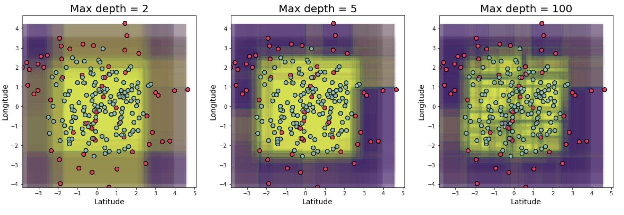
Bagging does well to reduce overfitting, but only upto a certain extent.
Vary the max_depth and numboot variables to see how Bagging helps reduce overfitting with the help of the visualization below
# We will make plots for three different values of `max_depth`

fig,axes = plt.subplots(1,3,figsize=(20,6))

# Make a list of three max_depths to investigate
max_depth = [2,5,100]

# Fix the number of bootstraps

numboot = 100

for index,ax in enumerate(axes):

    for i in range(numboot):
        df_new = df.sample(frac=1,replace=True)
        y = df_new.land_type.values
        X = df_new[['latitude', 'longitude']].values
        dtree = DecisionTreeClassifier(max_depth=max_depth[index])
        dtree.fit(X, y)
        ax.scatter(X[:, 0], X[:, 1], c=y-1, s=50,alpha=0.5,edgecolor="k",cmap=cmap_bold)
        plot_step_x1= 0.1
        plot_step_x2= 0.1
        x1min, x1max= X[:,0].min(), X[:,0].max()
        x2min, x2max= X[:,1].min(), X[:,1].max()
        x1, x2 = np.meshgrid(np.arange(x1min, x1max, plot_step_x1), np.arange(x2min, x2max, plot_step_x2) )
        # Re-cast every coordinate in the meshgrid as a 2D point
        Xplot= np.c_[x1.ravel(), x2.ravel()]

        # Predict the class
        y = dtree.predict( Xplot )
        y= y.reshape( x1.shape )
        cs = ax.contourf(x1, x2, y, alpha=0.02)


    ax.set_xlabel('Latitude',fontsize=14)
    ax.set_ylabel('Longitude',fontsize=14)
    ax.set_title(f'Max depth = {max_depth[index]}',fontsize=20)
Mindchow 🍲
Play around with the following parameters:
- max_depth
- numboot
Based on your observations, answer the questions below:
How does the plot change with varying
max_depthHow does the plot change with varying
numbootHow are the three plots essentially different?
Does more bootstraps reduce overfitting for
- High depth
- Low depth