Key Word(s): bagging
Instructions:
- Read the dataset airquality.csv as a pandas dataframe.
- Take a quick look at the dataset.
- Split the data into train and test sets.
- Specify the number of bootstraps as 30 and a maximum depth of 3.
- Define a Bagging Regression model that uses Decision Tree as its base estimator.
- Fit the model on the train data.
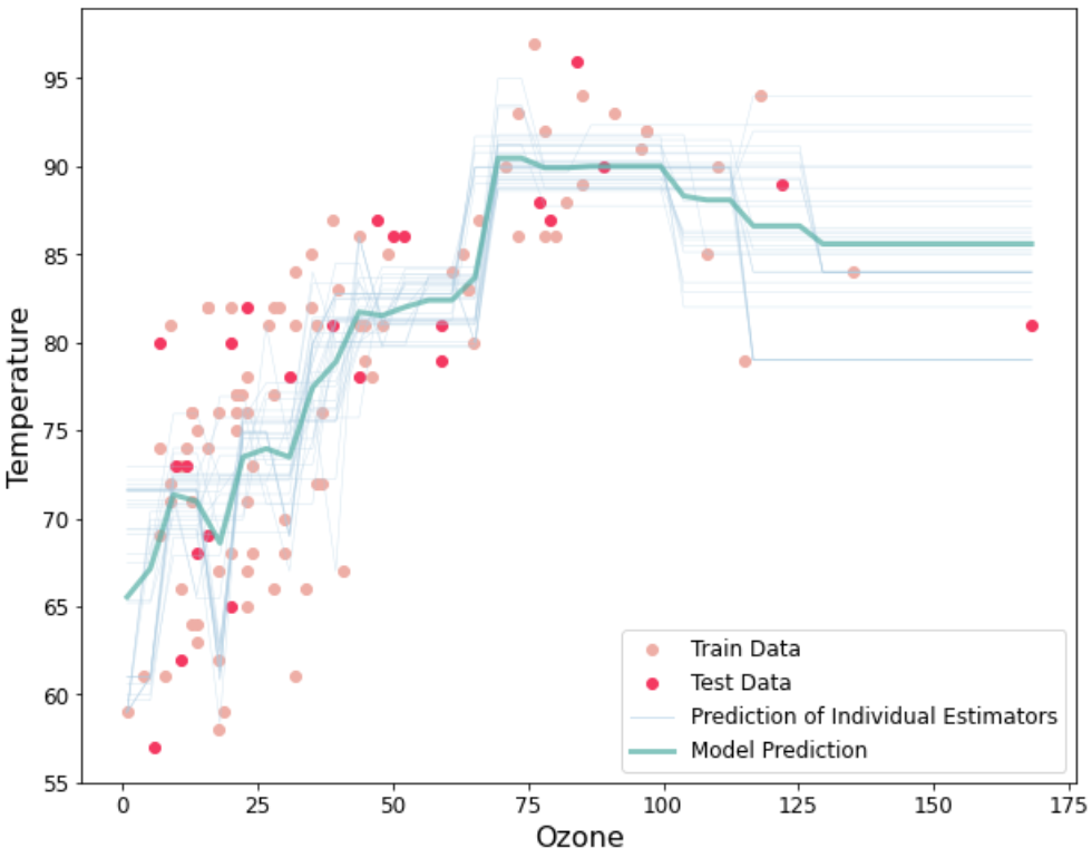
- Use the helper code to predict using the mean model and individual estimators. The plot will look similar to the one given above.
- Predict on the test data using the first estimator and the mean model.
- Compute and display the test MSEs.
Hints:
sklearn.train_test_split() : Split arrays or matrices into random train and test subsets.
BaggingRegressor() : Returns a Bagging regressor instance.
DecisionTreeRegressor() : A decision tree regressor.
DecisionTreeRegressor().estimators_ : A list of estimators. Use this to access any of the estimators.
sklearn.mean_squared_error() : Mean squared error regression loss.
In [2]:
# Import necessary libraries

import numpy as np
from numpy import mean
from numpy import std
from sklearn.datasets import make_regression
from sklearn.ensemble import BaggingRegressor
import matplotlib.pyplot as plt
import pandas as pd
import itertools
from sklearn.tree import DecisionTreeRegressor
from sklearn.metrics import mean_squared_error
from sklearn.model_selection import train_test_split
%matplotlib inline
In [3]:
# Read the dataset
df = pd.read_csv("airquality.csv",index_col=0)
In [10]:
# Take a quick look at the data
df.head(10)
In [12]:
# We will only use Ozone for this exerice. Drop any notnas
df = df[df.Ozone.notna()]
In [17]:
# Assign "x" column as the predictor variable, only use Ozone, and "y" as the
x = df[['Ozone']].values
y = df['Temp']
In [20]:
# Split the data into train and test sets with train size as 0.8 and random_state as 102
x_train, x_test, y_train, y_test = train_test_split(x, y, train_size=0.8, random_state=102)
Bagging Regressor
In [21]:
# Specify the number of bootstraps as 30
num_bootstraps = 30

# Specify the maximum depth of the decision tree as 3
max_depth = 3

# Define the Bagging Regressor Model
# Use Decision Tree as your base estimator with depth as mentioned in max_depth
# Initialise number of estimators using the num_bootstraps value
model = ___


# Fit the model on the train data
___
Out[21]:
In [24]:
# Helper code to plot the predictions of individual estimators and
plt.figure(figsize=(10,8))

xrange = np.linspace(x.min(),x.max(),80).reshape(-1,1)
plt.plot(x_train,y_train,'o',color='#EFAEA4', markersize=6, label="Train Data")
plt.plot(x_test,y_test,'o',color='#F6345E', markersize=6, label="Test Data")

plt.xlim()
for i in model.estimators_:
    y_pred1 = i.predict(xrange)
    plt.plot(xrange,y_pred1,alpha=0.5,linewidth=0.5,color = '#ABCCE3')
plt.plot(xrange,y_pred1,alpha=0.6,linewidth=1,color = '#ABCCE3',label="Prediction of Individual Estimators")


y_pred = model.predict(xrange)
plt.plot(xrange,y_pred,alpha=0.7,linewidth=3,color='#50AEA4', label='Model Prediction')
plt.xlabel("Ozone", fontsize=16)
plt.ylabel("Temperature", fontsize=16)
plt.xticks(fontsize=12)
plt.yticks(fontsize=12)
plt.legend(loc='best',fontsize=12)
plt.show()
In [25]:
# Compute the test MSE of the prediction of individual estimator
y_pred1 = ___
print("The test MSE of one estimator in the model is", round(mean_squared_error(y_test,y_pred1),2))
In [ ]:
### edTest(test_mse) ###
# Compute the test MSE of the model prediction
y_pred = ___
print("The test MSE of the model is",round(mean_squared_error(y_test,y_pred),2))
Mindchow 🍲
After marking, go back and change the number of bootstraps and the maximum depth of the tree.
Do you see any relation between them?
How does the variance change with change in maximum depth?
How does the variance change with change in number of bootstraps?
Your answer here
In [ ]: