Key Word(s): PCA

Title¶

Exercise - PCA

Description¶

The goal of the exercise is understand what a PCA decomposition is, how to implement it in sklearn, and how to use the results as predictors in a logistic regression model. You will produce a nice looking plot like this:

Instructions:¶

We are going to use the Heart dataset that we have seen before.

Load the Heart data set and define y and X.
Perform PCA decomposition on X, and better understand what it represents.
Plot the first two PCA components to see if separation of classes is possible
Fit the various PCR logistic models, and interpret the output.

sklearn.LogisticRegression() : Generates a Logistic Regression classifier

sklearn.PCA() : Fits the model to the given data

sklearn.StandardScaler() : Fits the model to the given data

Note: This exercise is auto-graded and you can try multiple attempts.

In [ ]:

%matplotlib inline
import sys
import numpy as np
import pylab as pl
import pandas as pd
import sklearn as sk
import statsmodels.api as sm
import matplotlib.pyplot as plt
import matplotlib
import seaborn as sns

from sklearn.linear_model import LogisticRegression
from sklearn.decomposition import PCA
import sklearn.metrics as met


pd.set_option('display.width', 500)
pd.set_option('display.max_columns', 100)

PCA¶

Part 0: Reading the data¶

In this notebook, we will be using the same Heart dataset from last lecture. As a reminder the variables we will be using today include:

AHD: whether or not the patient presents atherosclerotic heart disease (a heart attack): Yes or No
Sex: a binary indicator for whether the patient is male (Sex=1) or female (Sex=0)
Age: age of patient, in years
MaxHR: the maximum heart rate of patient based on exercise testing
RestBP: the resting systolic blood pressure of the patient
Chol: the HDL cholesterol level of the patient
Oldpeak: ST depression induced by exercise relative to rest (on an ECG)
Slope: the slope of the peak exercise ST segment (1 = upsloping; 2 = flat; 3 = downsloping)
Ca: number of major vessels (0-3) colored by flourosopy

For further information on the dataset, please see the UC Irvine Machine Learning Repository.

In [ ]:

df_heart = pd.read_csv('Heart.csv')

# Force the response into a binary indicator:
df_heart['AHD'] = 1*(df_heart['AHD'] == "Yes")

print(df_heart.shape)
df_heart.head()

Part 1: Principal Components Analysis (PCA)¶

Q1.1 Just a sidebar (and a curiosity), what happens when two of the identical predictor is used in logistic regression? Is an error created? Should one be? Investigate by predicting AHD from two copies of Age, and compare to the simple logistic regression model with Age alone.

In [ ]:

y = df_heart['AHD']

logit1 = LogisticRegression(penalty="none",solver="lbfgs").fit(df_heart[['Age']],y)

# investigating what happens when two identical predictors of 'Age' are used
logit2 = LogisticRegression(penalty="none",solver="lbfgs").fit(___,y)

print("The coef estimate for Age (when in the model once):",logit1.coef_)
print("The coef estimates for Age (when in the model twice):",logit2.coef_)

your answer here

We will apply PCA to the heart dataset when there are just 4 predictors considered (remember: PCA is used when dimensionality is high (lots of predictors), but this will help us get our heads around what is going on):

In [ ]:

# For pedagogical purposes, let's simplify our lives and use just 7 predictors
X = df_heart[['Age','RestBP','Chol','MaxHR','Sex','Oldpeak','Slope']]
y = df_heart['AHD']
X.describe()

In [ ]:

# Here is the table of correlations between our predictors.  This will be useful later on
X.corr()

Q1.2 Is there any evidence of multicollinearity in the set of predictors? How do you know? How will PCA handle these correlations?

your answer here

Next we apply the PCA transformation in a few steps, and show some of the results below:

In [ ]:

# create/fit the 'full' pca transformation
pca = PCA().fit(X)

# apply the pca transformation to the full predictor set
pcaX = pca.transform(X)

# convert to a data frame
pcaX_df = pd.DataFrame(pcaX, columns=[['PCA1' , 'PCA2', 'PCA3', 'PCA4', 'PCA5', 'PCA6', 'PCA7']])

# here are the weighting (eigen-vectors) of the variables (first 2 at least)
print("First PCA Component (w1):",pca.components_[0,:])
print("Second PCA Component (w2):",pca.components_[1,:])

# here is the variance explained:
print("Variance explained by each component:",pca.explained_variance_ratio_)

Q1.3 Now try the PCA decompositon on the standardized version of X instead.

In [ ]:

### edTest(test_pcaZ) ###

# create/fit the standardized version of X
Z = sk.preprocessing.StandardScaler().fit(___).transform(___)

# create/fit the 'full' pca transformation on Z
pca_standard = PCA().fit(___)
pcaZ = pca_standard.transform(___)

# convert to a data frame
pcaZ_df = pd.DataFrame(___, columns=[['PCA1' , 'PCA2', 'PCA3', 'PCA4', 'PCA5', 'PCA6', 'PCA7']])

In [ ]:

# Let's look at them to see what they are comprised of:
pd.DataFrame.from_dict({'Variable': X.columns,
                        'PCA1': pca.components_[0],
                        'PCA2': pca.components_[1],
                        'PCA-Z1': pca_standard.components_[0],
                        'PCA-Z2': pca_standard.components_[1]})

Q1.3 Interpret the results above. What doss $w_1$ represent based on the untransformed data? What doss $w_1$ represent based on the standardized data? Which is a better representation of the data?

your answer here

In [ ]:

np.sum(pca.components_[0,:]**2)

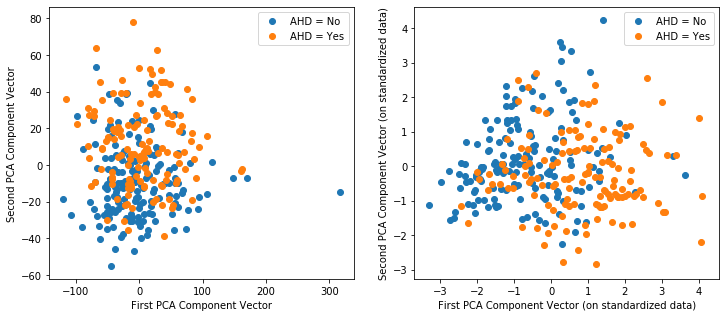
Q1.4 It is common for a model with high dimensional data (lots of predictors) to be plotted along the first 2 PCA components (with the classification boundaries added). Below is the scatter plot for these data (without a classificaiton boundary, since we do not have a model yet) for the unstandardized PCA. Repeat this for the standardized PCA:

In [ ]:

# Plot the response over the first 2 PCA component vectors

fig,(ax1,ax2) =  plt.subplots(1, 2, figsize = (12,5))

ax1.scatter(pcaX_df[['PCA1']][y==0],pcaX_df[['PCA2']][y==0])
ax1.scatter(pcaX_df[['PCA1']][y==1],pcaX_df[['PCA2']][y==1])
ax1.legend(["AHD = No","AHD = Yes"])
ax1.set_xlabel("First PCA Component Vector")
ax1.set_ylabel("Second PCA Component Vector");

Q2.4 Does there appear to be good potential here? Which form of the data appear to provide better information as to seperate the classes in the response? What at would a classification boundary look like if a logistic regression model were fit using the first 2 principal components as the predictors?

your answer here

Part 2: PCA in Regression (PCR)¶

First let's fit the full logistic regression model to predict AHD from the 7 predictors above.

Remember: PCA is an approach to handling the predictors (unsupervised), so it does not matter if we are using it for a regression or classification type problem.

In [ ]:

#fit the 'full' model on the 7 predictors. and print out the coefficients
logit_full = LogisticRegression(penalty="none",solver="lbfgs",max_iter=2000).fit(X,y)

beta = logit_full.coef_[0]

print(beta)

Q2.1 Fit the logistic model on the first PCA vector below and get some relevant output

In [ ]:

### edTest(test_pcr1) ###

logit_pcr1 = LogisticRegression(penalty = 'none', solver="lbfgs").fit(___,y)

print("Intercept from simple PCR-Logistic:",logit_pcr1.intercept_)
print("'Slope' from simple PCR-Logistic:", logit_pcr1.coef_)

print("First PCA Component (w1):",pca.components_[0:1,:])

Q2.2 What does this PCR-1 model tell us about how the predictors relate to the response (aka, estimate the coefficient(s) in the original predictor space)? Is it truly a simple logistic regression model in the original predictor space?

In [ ]:

# your code here: do a multiplication of pcr_1's coefficients times the first component vector from PCA

(logit_pcr1.coef_*pca.components_[0:1,:])

your answer here

Here is the above claculation fora few up to the 7th PCR logistic regression, and then plotted on a 'pretty' plot:

In [ ]:

# Fit the other 3 PCRs on the rest of the 7 predictors
#pcaX_df.iloc[:,np.arange(0,5)].head()

logit_pcr2 = LogisticRegression(C=1000000,solver="lbfgs").fit(pcaX_df[['PCA1','PCA2']],y)
logit_pcr3 = LogisticRegression(C=1000000,solver="lbfgs").fit(pcaX_df[['PCA1','PCA2','PCA3']],y)
logit_pcr4 = LogisticRegression(C=1000000,solver="lbfgs").fit(pcaX_df[['PCA1','PCA2','PCA3','PCA4']],y)
logit_pcr5 = LogisticRegression(C=1000000,solver="lbfgs").fit(pcaX_df[['PCA1','PCA2','PCA3','PCA4','PCA5']],y)
logit_pcr6 = LogisticRegression(C=1000000,solver="lbfgs").fit(pcaX_df[['PCA1','PCA2','PCA3','PCA4','PCA5','PCA6']],y)
logit_pcr7 = LogisticRegression(C=1000000,solver="lbfgs").fit(pcaX_df,y)

pcr1=(logit_pcr1.coef_*np.transpose(pca.components_[0:1,:])).sum(axis=1)
pcr2=(logit_pcr2.coef_*np.transpose(pca.components_[0:2,:])).sum(axis=1)
pcr3=(logit_pcr3.coef_*np.transpose(pca.components_[0:3,:])).sum(axis=1)
pcr4=(logit_pcr4.coef_*np.transpose(pca.components_[0:4,:])).sum(axis=1)
pcr5=(logit_pcr5.coef_*np.transpose(pca.components_[0:5,:])).sum(axis=1)
pcr6=(logit_pcr6.coef_*np.transpose(pca.components_[0:6,:])).sum(axis=1)
pcr7=(logit_pcr7.coef_*np.transpose(pca.components_[0:7,:])).sum(axis=1)

results = np.vstack((pcr1,pcr2,pcr3,pcr4,pcr5,pcr6,pcr7,beta))
print(results)

In [ ]:

plt.plot(['PCR1','PCR2', 'PCR3', 'PCR4','PCR5','PCR6','PCR7', 'Logistic'],results)

plt.ylabel("Back-calculated Beta Coefficients");

#plt.legend(X.columns);

Q2.3 Interpret the plot above. Specifically, compare how each PCA vector "contributes" to the original logistic regression model using all 7 original predictors. How Does PCR-4 compare to the original logistic regression model (in estimated coefficients)?

your answer here

All of this PCA work should have been done using the standardized versions of the predictors. Below is the code that does exactly that:

In [ ]:

scaler = sk.preprocessing.StandardScaler()
scaler.fit(X)
Z = scaler.transform(X)
pca = PCA(n_components=7).fit(Z)
pcaZ = pca.transform(Z)
pcaZ_df = pd.DataFrame(pcaZ, columns=[['PCA1' , 'PCA2', 'PCA3', 'PCA4','PCA5', 'PCA6', 'PCA7']])

print("First PCA Component (w1):",pca.components_[0,:])
print("Second PCA Component (w2):",pca.components_[1,:])

In [ ]:

#fit the 'full' model on the 4 predictors. and print out the coefficients
logit_full = LogisticRegression(C=1000000,solver="lbfgs").fit(Z,y)


betaZ = logit_full.coef_[0]

print("Logistic coef. on standardized predictors:",betaZ)

In [ ]:

# Fit the PCR
logit_pcr1Z = LogisticRegression(C=1000000,solver="lbfgs").fit(pcaZ_df[['PCA1']],y)
logit_pcr2Z = LogisticRegression(C=1000000,solver="lbfgs").fit(pcaZ_df[['PCA1','PCA2']],y)
logit_pcr3Z = LogisticRegression(C=1000000,solver="lbfgs").fit(pcaZ_df[['PCA1','PCA2','PCA3']],y)
logit_pcr4Z = LogisticRegression(C=1000000,solver="lbfgs").fit(pcaZ_df[['PCA1','PCA2','PCA3','PCA4']],y)
logit_pcr7Z = LogisticRegression(C=1000000,solver="lbfgs").fit(pcaZ_df,y)

pcr1Z=(logit_pcr1Z.coef_*np.transpose(pca.components_[0:1,:])).sum(axis=1)
pcr2Z=(logit_pcr2Z.coef_*np.transpose(pca.components_[0:2,:])).sum(axis=1)
pcr3Z=(logit_pcr3Z.coef_*np.transpose(pca.components_[0:3,:])).sum(axis=1)
pcr4Z=(logit_pcr4Z.coef_*np.transpose(pca.components_[0:4,:])).sum(axis=1)
pcr7Z=(logit_pcr7Z.coef_*np.transpose(pca.components_)).sum(axis=1)

resultsZ = np.vstack((pcr1Z,pcr2Z,pcr3Z,pcr4Z,pcr7Z,betaZ))
print(resultsZ)

plt.plot(['PCR1-Z' , 'PCR2-Z', 'PCR3-Z', 'PCR4-Z', 'PCR7-Z', 'Logistic'],resultsZ)

plt.ylabel("Back-calculated Beta Coefficients");

plt.legend(X.columns);

Q2.4 Compare this plot to the previous one; why does this plot make sense?. What does this illustrate?

your answer here

In [ ]: