Key Word(s): Logistic Regression, Classification
Instructions:
We are trying to predict the types of Irises in the classic Iris data set based on measured characteristics
- Load the Iris data set and convert to a data frame.
- Fit multinomial & OvR logistic regressions and a $k$-NN model.
- Compute the accuracy of the models.
- Plot the classification boundaries against the two predictors used.
Hints:
sklearn.LogisticRegression() : Generates a Logistic Regression classifier
sklearn.fit() : Fits the model to the given data
sklearn.predict() : Predict using the estimated model (Logistic or knn classifiers) to perform pure classification predictions
sklearn.predict_proba() : Predict using the estimated model (Logistic or knn classifiers) to perform probability predictions of all the classes in the response (they should add up to 1 for each observation)
sklearn.LogisticRegression.coef_ and .intercept_ : Pull off the estimated $\beta$ coefficients in a Logistic Regression model
sklearn.score() : Accuracy classification score.
matplotlib.pcolormesh() : Accuracy classification score
Note: This exercise is auto-graded and you can try multiple attempts.
%matplotlib inline
from sklearn import datasets
import matplotlib.pyplot as plt
import seaborn as sns
import pandas as pd
import numpy as np
from sklearn.linear_model import LogisticRegression
from sklearn.neighbors import KNeighborsClassifier
Irises
Read in the data set and convert to a Pandas data frame:
raw = datasets.load_iris()
iris = pd.DataFrame(raw['data'],columns=raw['feature_names'])
iris['type'] = raw['target']
iris.head()
Note: this violin plot is 'inverted': putting the response variable in the model on the x-axis. This is fine for exploration
sns.violinplot(y=iris['sepal length (cm)'], x=iris['type'], split=True);
# Create a violin plot to compare petal length
# across the types of irises

sns.violinplot(___);
Here we fit our first model (the OvR logistic) and print out the coefficients:
logit_ovr = LogisticRegression(penalty='none', multi_class='ovr',max_iter = 1000).fit(
    iris[['sepal length (cm)','sepal width (cm)']], iris['type'])
print(logit_ovr.intercept_)
print(logit_ovr.coef_)
# we can predict classes or probabilities
print(logit_ovr.predict(iris[['sepal length (cm)','sepal width (cm)']])[0:5])
print(logit_ovr.predict_proba(iris[['sepal length (cm)','sepal width (cm)']])[0:5])
# and calculate accuracy
print(logit_ovr.score(iris[['sepal length (cm)','sepal width (cm)']],iris['type']))
Now it's your turn: but this time with the multinomial logistic regression.
### edTest(test_multinomial) ###

# Fit the model and print out the coefficients
logit_multi = LogisticRegression(___).fit(___)
intercept = logit_multi.intercept_
coefs = logit_multi.coef_
print(intercept)
print(coefs)
### edTest(test_multinomialaccuracy) ###

multi_accuracy = ___
print(multi_accuracy)
# Plot the decision boundary.
x1_range = iris['sepal length (cm)'].max() - iris['sepal length (cm)'].min()
x2_range = iris['sepal width (cm)'].max() - iris['sepal width (cm)'].min()
x1_min, x1_max = iris['sepal length (cm)'].min()-0.1*x1_range, iris['sepal length (cm)'].max() +0.1*x1_range
x2_min, x2_max = iris['sepal width (cm)'].min()-0.1*x2_range, iris['sepal width (cm)'].max() + 0.1*x2_range

step = .05
x1x, x2x = np.meshgrid(np.arange(x1_min, x1_max, step), np.arange(x2_min, x2_max, step))
y_hat_ovr = logit_ovr.predict(np.c_[x1x.ravel(), x2x.ravel()])
y_hat_multi = ___


fig, (ax1, ax2) = plt.subplots(1, 2,  figsize=(15, 6))

ax1.pcolormesh(x1x, x2x, y_hat_ovr.reshape(x1x.shape), cmap=plt.cm.Paired,alpha = 0.5)
ax1.scatter(iris['sepal length (cm)'], iris['sepal width (cm)'], c=iris['type'], edgecolors='k', cmap=plt.cm.Paired)

### your job is to create the same plot, but for the multinomial
#####
# your code here
#####

plt.show()
#fit a knn model (k=5) for the same data
knn5 = KNeighborsClassifier(___).fit(___)
### edTest(test_knnaccuracy) ###

#Calculate the accuracy
knn5_accuracy = ___
print(knn5_accuracy)
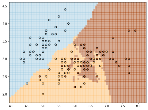
# and plot the classification boundary

y_hat_knn5 = knn5.predict(np.c_[x1x.ravel(), x2x.ravel()])

fig, ax1 = plt.subplots(1, 1,  figsize=(8, 6))

ax1.pcolormesh(x1x, x2x, y_hat_knn5.reshape(x1x.shape), cmap=plt.cm.Paired,alpha = 0.5)
# Plot also the training points
ax1.scatter(iris['sepal length (cm)'], iris['sepal width (cm)'], c=iris['type'], edgecolors='k', cmap=plt.cm.Paired)

plt.show()