Title¶

Exercise: 1 - Regularization with Cross-validation

Description¶

The aim of this exercise is to understand regularization with cross-validation.

Instructions:¶

Initialising the required parameters for this exercise. This can be viewed in the scaffold.
Read the data file polynomial50.csv and assign the predictor and response variables.
Use the helper code to visualise the data.
Define a function reg_with_validation that performs Ridge regularization by taking a random_state parameter.
- Split the data into train and validation sets by specifying the random_state.
- Compute the polynomial features for the train and validation sets.
- Run a loop for the alpha values. Within the loop:
  - Initialise the Ridge regression model with the specified alpha.
  - Fit the model on the training data and predict and on the train and validation set.
  - Compute the MSE of the train and validation prediction.
  - Store these values in lists.
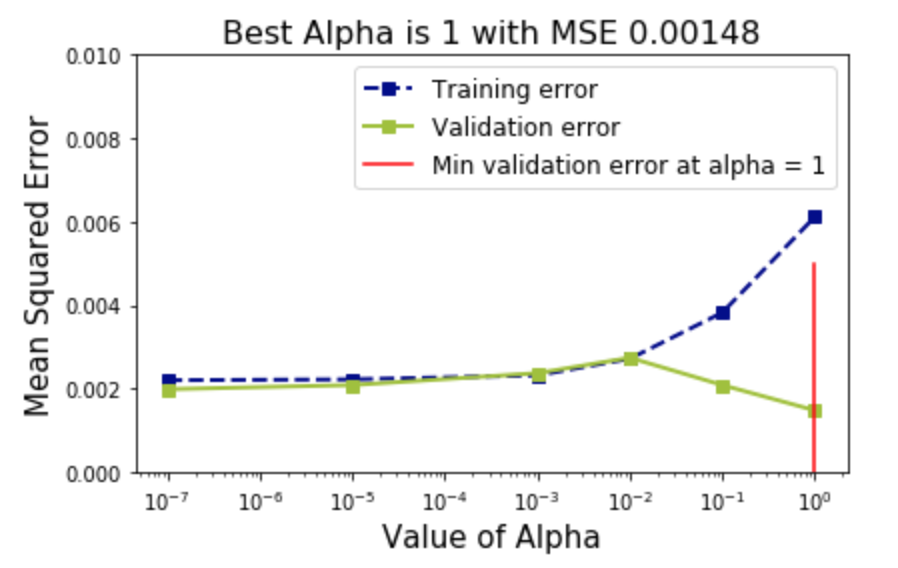
Run reg_with_validation for varying random states and plot a graph that depicts the best alpha value and the best MSE. The graph will be similar to the one given above.
Define a function reg_with_cross_validation that performs Ridge regularization with cross-validation by taking a random_state parameter.
- Sample the data using the specified random state.
- Assign the predictor and response variables using the sampled data.
- Run a loop for the alpha values. Within the loop:
  - Initialise the Ridge regression model with the specified alpha.
  - Fit the model on the entire data and using cross-validation with 5 folds.
  - Get the train and validation MSEs by taking their mean.
  - Store these values in lists.
Run reg_with_cross_validation for varying random states and plot a graph that depicts the best alpha value and the best MSE.
Use the helper code given to print your best MSEs in the case of simple validation and cross-validation for different random states.

Hints:¶

df.sample() : Returns a random sample of items from an axis of the object.

sklearn.cross_validate() : Evaluate metrics by cross-validation and also record fit/score times.

np.mean() : Compute the arithmetic mean along the specified axis.

sklearn.RidgeRegression() : Linear least squares with l2 regularization.

sklearn.fit() : Fit Ridge egression model.

sklearn.predict() : Predict using the linear model.

sklearn.mean_squared_error() : Mean squared error regression loss

sklearn.PolynomialFeatures() : Generate polynomial and interaction features.

sklearn.fit_transform() : Fit to data, then transform it.

In [ ]:

# Import required libraries

import numpy as np
import pandas as pd
import matplotlib.pyplot as plt
from prettytable import PrettyTable
from sklearn.model_selection import train_test_split
from sklearn.preprocessing import PolynomialFeatures
from sklearn.metrics import mean_squared_error
from sklearn.linear_model import Ridge
from sklearn.model_selection import cross_validate
%matplotlib inline

In [ ]:

# Initialising required parameters

# The list of random states
ran_state = [0, 10, 21, 42, 66, 109, 310, 1969]

# The list of alpha for regularization
alphas = [1e-7,1e-5, 1e-3, 0.01, 0.1, 1]

# The degree of the polynomial
degree= 30

In [ ]:

# Read the file 'polynomial50.csv' as a dataframe
df = pd.read_csv('polynomial50.csv')

# Assign the values of the 'x' column as the predictor
x = df[['x']].values

# Assign the values of the 'y' column as the response
y = df['y'].values

# Also assign the true value of the function (column 'f') to the variable f 
f = df['f'].values

In [ ]:

# Use the helper code below to visualise the distribution of the x, y values & also the value of the true function f

fig, ax = plt.subplots()

# Plot x vs y values
ax.plot(x,y, 'o', label = 'Observed values',markersize=10 ,color = 'Darkblue')

# Plot x vs true function value
ax.plot(x,f, 'k-', label = 'True function',linewidth=4,color ='#9FC131FF')

ax.legend(loc = 'best');
ax.set_xlabel('Predictor - $X$',fontsize=16)
ax.set_ylabel('Response - $Y$',fontsize=16)
ax.set_title('Predictor vs Response plot',fontsize=16);

In [ ]:

# Function to perform regularization with simple validation
def reg_with_validation(rs):
    
    # Split the data into train and validation sets with train size as 80% and random_state as
    x_train, x_val, y_train, y_val = train_test_split(x,y, train_size = 0.8, random_state=rs)

    # Create two lists for training and validation error
    training_error, validation_error = [],[]

    # Compute the polynomial features train and validation sets
    x_poly_train = ___
    x_poly_val= ___

    # Run a loop for all alpha values
    for alpha in alphas:

        # Initialise a Ridge regression model by specifying the alpha and with fit_intercept=False
        ridge_reg = ___
        
        # Fit on the modified training data
        ___

        # Predict on the training set 
        y_train_pred = ___
        
        # Predict on the validation set 
        y_val_pred = ___
        
        # Compute the training and validation mean squared errors
        mse_train = ___
        mse_val = ___

        # Append the MSEs to their respective lists 
        training_error.append(mse_train)
        validation_error.append(mse_val)
    
    # Return the train and validation MSE
    return training_error, validation_error

In [ ]:

### edTest(test_validation) ###
# Initialise a list to store the best alpha using simple validation for varying random states
best_alpha = []

# Run a loop for different random_states
for i in range(len(ran_state)):
    
    # Get the train and validation error by calling the function reg_with_validation
    training_error, validation_error = ___

    # Get the best mse from the validation_error list
    best_mse  = ___
    
    # Get the best alpha value based on the best mse
    best_parameter = ___
    
    # Append the best alpha to the list
    best_alpha.append(best_parameter)
    
    # Use the helper code given below to plot the graphs
    fig, ax = plt.subplots(figsize = (6,4))
    
    # Plot the training errors for each alpha value
    ax.plot(alphas,training_error,'s--', label = 'Training error',color = 'Darkblue',linewidth=2)
    
    # Plot the validation errors for each alpha value
    ax.plot(alphas,validation_error,'s-', label = 'Validation error',color ='#9FC131FF',linewidth=2 )

    # Draw a vertical line at the best parameter
    ax.axvline(best_parameter, 0, 0.75, color = 'r', label = f'Min validation error at alpha = {best_parameter}')

    ax.set_xlabel('Value of Alpha',fontsize=15)
    ax.set_ylabel('Mean Squared Error',fontsize=15)
    ax.set_ylim([0,0.010])
    ax.legend(loc = 'best',fontsize=12)
    bm = round(best_mse, 5)
    ax.set_title(f'Best alpha is {best_parameter} with MSE {bm}',fontsize=16)
    ax.set_xscale('log')
    plt.tight_layout()
    plt.show()

In [ ]:

# Function to perform regularization with cross validation
def reg_with_cross_validation(rs):
    
    # Sample your data to get different splits using the random state
    df_new = ___
    
    # Assign the values of the 'x' column as the predictor from your sampled dataframe
    x = df_new[['x']].values

    # Assign the values of the 'y' column as the response from your sampled dataframe
    y = df_new['y'].values

    # Create two lists for training and validation error
    training_error, validation_error = [],[]

    # Compute the polynomial features on the entire data
    x_poly = ___

    # Run a loop for all alpha values
    for alpha in alphas:

        # Initialise a Ridge regression model by specifying the alpha value and with fit_intercept=False
        ridge_reg = ___
        
        # Perform cross validation on the modified data with neg_mean_squared_error as the scoring parameter and cv=5
        # Remember to get the train_score
        ridge_cv = ___

        # Compute the training and validation errors got after cross validation
        mse_train = ___
        mse_val = ___
        
        # Append the MSEs to their respective lists 
        training_error.append(mse_train)
        validation_error.append(mse_val)
    
    # Return the train and validation MSE
    return training_error, validation_error

In [ ]:

### edTest(test_cross_validation) ###
# Initialise a list to store the best alpha using cross validation for varying random states
best_cv_alpha = []

# Run a loop for different random_states
for i in range(len(ran_state)):
    
    # Get the train and validation error by calling the function reg_with_cross_validation
    training_error, validation_error = ___
    
    # Get the best mse from the validation_error list
    best_mse  = ___
    
    # Get the best alpha value based on the best mse
    best_parameter = ___
    
    # Append the best alpha to the list
    best_cv_alpha.append(best_parameter)
    
    # Use the helper code given below to plot the graphs
    fig, ax = plt.subplots(figsize = (6,4))
    
    # Plot the training errors for each alpha value
    ax.plot(alphas,training_error,'s--', label = 'Training error',color = 'Darkblue',linewidth=2)
    
    # Plot the validation errors for each alpha value
    ax.plot(alphas,validation_error,'s-', label = 'Validation error',color ='#9FC131FF',linewidth=2 )

    # Draw a vertical line at the best parameter
    ax.axvline(best_parameter, 0, 0.75, color = 'r', label = f'Min validation error at alpha = {best_parameter}')

    ax.set_xlabel('Value of Alpha',fontsize=15)
    ax.set_ylabel('Mean Squared Error',fontsize=15)
    ax.legend(loc = 'best',fontsize=12)
    bm = round(best_mse, 5)
    ax.set_title(f'Best alpha is {best_parameter} with MSE {bm}',fontsize=16)
    ax.set_xscale('log')
    plt.tight_layout()

In [ ]:

# Use the helper code below to print your findings
pt = PrettyTable()

pt.field_names = ["Random State", "Best Alpha with Validation", "Best Alpha with Cross-Validation"]

for i in range(6):
    pt.add_row([ran_state[i], best_alpha[i], best_cv_alpha[i]])

print(pt)

What can you infer about cross-validation based on the previous analysis?

After marking, change the random states and alpha values. Run the code again. Comment on the results of regularization with simple validation and cross-validation.