Key Word(s): ridge, lasso, hyperparameters

Title¶

Exercise: 2 - Variation of coefficients

Description¶

The goal of this exercise is to understand the variation of the coefficients of the predictors with varying values of regularization parameter in Lasso and Ridge regularization.

Below is a sample plot for Ridge ($L_2$ regularization)

Instructions:¶

Read the dataset bateria_train.csv and assign the predictor and response variables.
The predictor is the Spreading factor and the response variable is the Perc_population
Use a maximum degree of 7 to make polynomial features and make a new predictor x_poly
Make a list of alpha values.
For each value of $\alpha$:
- Fit a multi-linear regression using $L_2$ regularization
- Compute the coefficient of the predictors and store to the plot later
Make a plot of the coefficients along with the alpha values
Make a new alpha list as per the code in the exercise
Implement Lasso regularization by repeating the above steps for each value of alpha
make another plot of the coefficients along with the new alpha values

Hints:¶

np.transpose() : Reverse or permute the axes of an array; returns the modified array

sklearn.normalize() : Scales input vectors individually to the unit norm (vector length)

sklearn.train_test_split() : Splits the data into random train and test subsets

sklearn.PolynomialFeatures() : Generates a new feature matrix consisting of all polynomial combinations of the features with degree less than or equal to the specified degree

sklearn.fit_transform() : Fits transformer to X and y with optional parameters fit_params and returns a transformed version of X

sklearn.LinearRegression() : LinearRegression fits a linear model

sklearn.fit() : Fits the linear model to the training data

sklearn.predict() : Predict using the linear modReturns the coefficient of the predictors in the model.

mean_squared_error() : Mean squared error regression loss

sklearn.coef_ : Returns the coefficients of the predictors

plt.subplots() : Create a figure and a set of subplots

ax.barh() : Make a horizontal bar plot

ax.set_xlim() : Sets the x-axis view limits

sklearn.Lasso() : Linear Model trained with L1 prior as a regularizer

sklearn.Ridge() : Linear least squares with L2 regularization

zip() : Makes an iterator that aggregates elements from each of the iterables.

Note: This exercise is auto-graded and you can try multiple attempts.

In [ ]:

# Import libraries

%matplotlib inline
import pandas as pd
import numpy as np
import matplotlib.pyplot as plt
from sklearn.linear_model import Lasso
from sklearn.linear_model import Ridge
from sklearn.preprocessing import PolynomialFeatures

In [ ]:

# Run this cell for more readable visuals 

large = 22; med = 16; small = 10
params = {'axes.titlesize': large,
          'legend.fontsize': med,
          'figure.figsize': (16, 10),
          'axes.labelsize': med,
          'axes.titlesize': med,
          'axes.linewidth': 2,
          'xtick.labelsize': med,
          'ytick.labelsize': med,
          'figure.titlesize': large}
plt.style.use('seaborn-white')
plt.rcParams.update(params)
#sns.set_style("white")
%matplotlib inline

In [ ]:

# Read the file "bacteria_train.csv" as a dataframe
# The file is the same as your homework 2

df = pd.read_csv("bacteria_train.csv")

In [ ]:

# Take a quick look of your dataset

df.head()

In [ ]:

# Store the predictor ('Spreading_factor') and the response ('Perc_population') values as the variables 'x' and 'y'

x, y  = df[[___]], df[___]

In [ ]:

# Select the number of polynomial features as per the maximum degree

maxdeg = 4
x_poly = PolynomialFeatures(___).fit_transform(___)

In [ ]:

# Select a list of alpha values ranging from 10 to 120 with 1000 points between them

alpha_list = np.linspace(___,___,___)
len(alpha_list)

In [ ]:

### edTest(test_ridge_fit) ###
# Make an empty list called coeff_list and for each alpha value, compute the coefficients and add it to coeff_list
coeff_list = []


#Now, you will implement the ridge regularisation for each alpha value, make sure you set Normalize=True

for i in alpha_list:

    ridge_reg = Ridge(alpha=___,normalize=___)

    #Fit on the entire data because we just want to see the trend of the coefficients

    ridge_reg.fit(___, ___)
    
    # Append the coeff_list with the coefficients of the model
    
    coeff_list.append(___)

In [ ]:

# We take the transpose of the list to get the variation in the coefficient values per degree

trend = np.array(coeff_list).T

In [ ]:

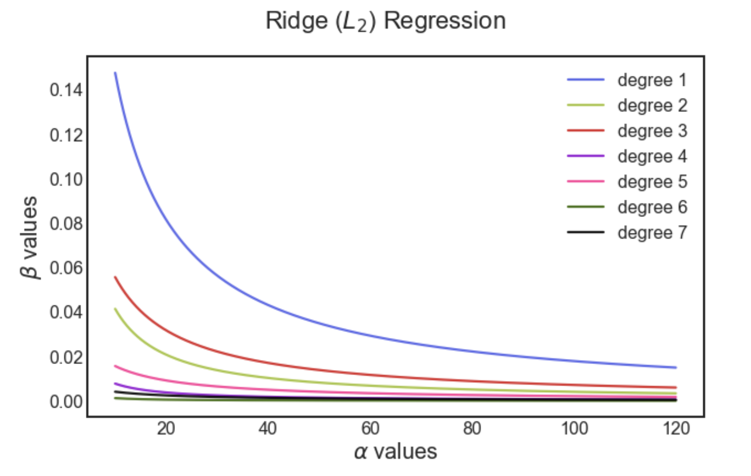
# Use the code below to plot the variation of the coefficients as per the alpha value

# Just adding some nice colors. make sure to comment this cell out if you plan to use degree more than 7
colors = ['#5059E8','#9FC131FF','#D91C1C','#9400D3','#FF2F92','#336600','black']

fig, ax = plt.subplots(figsize = (10,6))
for i in range(maxdeg):
    ax.plot(alpha_list,np.abs(trend[i+1]),color=colors[i],alpha = 0.9,label = f'Degree {i+1}',lw=2.2)
    ax.legend(loc='best',fontsize=10)
    ax.set_xlabel(r'$\alpha$ values', fontsize=20)
    ax.set_ylabel(r'$\beta$ values', fontsize=20)

fig.suptitle(r'Ridge ($L_2$) Regression');

Compare the results of Ridge regression with the Lasso variant¶

In [ ]:

# Select a list of alpha values ranging from 1e-4 to 1e-1 with 1000 points between them

alpha_list = np.linspace(___,___,___)
len(alpha_list)

In [ ]:

### edTest(test_lasso_fit) ###
# Make an empty list called coeff_list and for each alpha value, compute the coefficients and add it to coeff_list
coeff_list = []


#Now, you will implement the ridge regularisation for each alpha value, again normalize

for i in alpha_list:

    lasso_reg = Lasso(alpha=i,max_iter=250000,normalize=___)

    #Fit on the entire data because we just want to see the trend of the coefficients
    
    lasso_reg.fit(___, ___)
    
    # Again append the coeff_list with the coefficients of the model
    
    coeff_list.append(___)

In [ ]:

# We take the transpose of the list to get the variation in the coefficient values per degree

trend = np.array(coeff_list).T

In [ ]:

# Use helper code below to plot the variation of the coefficients as per the alpha value

colors = ['#5059E8','#9FC131FF','#D91C1C','#9400D3','#FF2F92','#336600','black']

fig, ax = plt.subplots(figsize = (10,6))
for i in range(maxdeg):
    ax.plot(alpha_list,np.abs(trend[i+1]),color=colors[i],alpha = 0.9,label = f'Degree {i+1}',lw=2)
    ax.legend(loc='best',fontsize=10)
    ax.set_xlabel(r'$\alpha$ values', fontsize=20)
    ax.set_ylabel(r'$\beta$ values', fontsize=20)

fig.suptitle(r'Lasso ($L_1$) Regression');

Mindchow 🍲¶

After marking the exercise, go back and change your maximum degree, and see how your coefficients vary for higher degrees

Remember to hide your colors variable to avoid index error while plotting coefficients

Your answer here

Now set the normalize=False. Things look different. Try to think why - Hint think of colinearity.

In [ ]: