Key Word(s): regularization, bias/variance trade-off, lasso, ridge
Instructions:
- Read the dataset and assign the predictor and response variables.
- Split the dataset into train and validation sets
- Fit a multi-linear regression model
- Compute the validation MSE of the model
- Compute the coefficient of the predictors and store to the plot later
- Implement Lasso regularization by specifying an alpha value. Repeat steps 4 and 5
- Implement Ridge regularization by specifying the same alpha value. Repeat steps 4 and 5
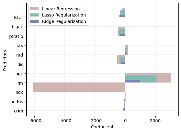
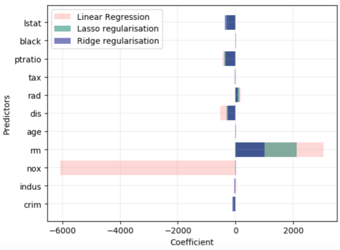
- Plot the coefficient of all the 3 models in one graph as shown above
Hints:
np.transpose() : Reverse or permute the axes of an array; returns the modified array
sklearn.normalize() : Scales input vectors individually to the unit norm (vector length)
sklearn.train_test_split() : Splits the data into random train and test subsets
sklearn.PolynomialFeatures() : Generates a new feature matrix consisting of all polynomial combinations of the features with degree less than or equal to the specified degree
sklearn.fit_transform() : Fits transformer to X and y with optional parameters fit_params and returns a transformed version of X
sklearn.LinearRegression() : LinearRegression fits a linear model
sklearn.fit() : Fits the linear model to the training data
sklearn.predict() : Predict using the linear modReturns the coefficient of the predictors in the model.
mean_squared_error() : Mean squared error regression loss
sklearn.coef_ : Returns the coefficients of the predictors
plt.subplots() : Create a figure and a set of subplots
ax.barh() : Make a horizontal bar plot
ax.set_xlim() : Sets the x-axis view limits
sklearn.Lasso() : Linear Model trained with L1 prior as a regularizer
sklearn.Ridge() : Linear least squares with L2 regularization
zip() : Makes an iterator that aggregates elements from each of the iterables.
Note: This exercise is auto-graded and you can try multiple attempts.
# Import libraries
%matplotlib inline
import pandas as pd
import numpy as np
import matplotlib.pyplot as plt
from sklearn import preprocessing
from sklearn.linear_model import Lasso
from sklearn.linear_model import Ridge
from sklearn.metrics import mean_squared_error
from sklearn.linear_model import LinearRegression
from sklearn.model_selection import train_test_split
from sklearn.preprocessing import PolynomialFeatures
Reading the dataset
# Read the file "Boston_housing.csv" as a dataframe

df = pd.read_csv("Boston_housing.csv")
df.head()
# Select a subdataframe of predictors mentioned above

X = df[___]

# Normalize the values of the dataframe

X_norm = preprocessing.normalize(___)

# Select medv as the response variable

y = df[___]
Split the dataset into train and validation sets
Keep the test size as 30% of the dataset, and use random_state=31
### edTest(test_random) ###
# Split the data into train and validation sets

X_train, X_val, y_train, y_val = train_test_split(___)
Multi-linear Regression Analysis
#Fit a linear regression model on the training data

lreg = LinearRegression()
lreg.fit(___)

# Predict on the validation set

y_val_pred = lreg.predict(___)
Computing the MSE for Multi-Linear Regression
# Use the mean_squared_error function to compute the validation mse

mse = mean_squared_error(___,___)

# print the MSE value

print ("Multi-linear regression validation MSE is", mse)
Obtaining the coefficients of the predictors
#make a dictionary of the coefficients along with the predictors as keys

lreg_coef = dict(zip(X.columns, np.transpose(lreg.coef_)))

#Linear regression coefficient values to plot

lreg_x = list(lreg_coef.keys())
lreg_y = list(lreg_coef.values())
Implementing Lasso regularization
# Now, you will implement the lasso regularisation

# Use alpha = 0.001

lasso_reg = Lasso(___)

#Fit on training data

lasso_reg.fit(___)

#Make a prediction on the validation data using the above trained model

y_val_pred =lasso_reg.predict(___)
Computing the MSE with Lasso regularization
# Again, calculate the validation MSE & print it

mse_lasso = mean_squared_error(___,___)

print ("Lasso validation MSE is", mse_lasso)
Obtaining the coefficients of the predictors
# Use the helper code below to make a dictionary of the predictors along with the coefficients associated with them

lasso_coef = dict(zip(X.columns, np.transpose(lasso_reg.coef_)))

#Lasso regularisation coefficient values to plot

lasso_x = list(lasso_coef.keys())
lasso_y = list(lasso_coef.values())
Implementing Ridge regularization
# Now, we do the same as above, but we use L2 regularisation

# Again, use alpha=0.001

ridge_reg = Ridge(___)

#Fit the model in the training data
ridge_reg.fit(___)

#Predict the model on the validation data
y_val_pred = ridge_reg.predict(___)
Computing the MSE with Ridge regularization
### edTest(test_mse) ###

# Calculate the validation MSE & print it

mse_ridge = mean_squared_error(___,___)
print ("Ridge validation MSE is", mse_ridge)
Obtaining the coefficients of the predictors
# Use the helper code below to make a dictionary of the predictors along with the coefficients associated with them

ridge_coef = dict(zip(X.columns, np.transpose(ridge_reg.coef_)))

#Ridge regularisation coefficient values to plot

ridge_x = list(ridge_coef.keys())
ridge_y = list(ridge_coef.values())
Plotting the graph
# Use the helper code below to visualise your results

plt.rcdefaults()

plt.barh(lreg_x,lreg_y,1.0, align='edge',color="#D3B4B4", label="Linear Regression")
plt.barh(lasso_x,lasso_y,0.75 ,align='edge',color="#81BDB2",label = "Lasso regularisation")
plt.barh(ridge_x,ridge_y,0.25 ,align='edge',color="#7E7EC0", label="Ridge regularisation")
plt.grid(linewidth=0.2)
plt.xlabel("Coefficient")
plt.ylabel("Predictors")
plt.legend(loc='best')

plt.show()
Compare the results of linear regression with that of lasso and ridge regularization.
Your answer here
After marking, change the alpha values to 1, 10 and 1000. What happens to the coefficients when alpha increases?
Your answer here