Key Word(s): hypothesis testing, confidence intervals

Title¶

Exercise: 1 - Hypothesis testing

Description¶

The goal of this exercise is to identify the relevant features of the dataset using Hypothesis testing and plotting a bar plot like the one below:

Instructions:¶

What we have done for you. Quickly review and observe the distributions of the coefficients:
Read the file Advertising.csv as a dataframe.
Fit a simple multi-linear regression with "medv" as the response variable and the remaining columns as the predictor variables.
Compute the coefficients of the model and plot a bar chart to depict these values.
To find the distributions of the coefficients

Your task:¶

Perform bootstrap.
For each bootstrap:
- Fit a simple multi-linear regression with the same conditions as before.
- Compute the coefficient values and store as a list.
Compute the ∣t∣ values for each of the coefficient value in the list.
Plot a bar chart of the varying ∣t∣ values.
Compute the p-value from the ∣t∣ values.
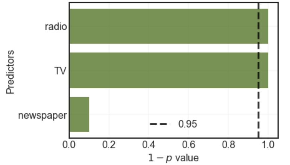
Plot a bar chart of 1−p values of the coefficients. Also mark the 0.95 line on the chart as shown above.

Hints:¶

sklearn.preprocessing.normalize() : Scales input vectors individually to unit norm (vector length).

np.interp() : Returns one-dimensional linear interpolation

df.sample() : Get a new sample from a dataframe

sklearn.LinearRegression() : LinearRegression fits a linear model

sklearn.fit() : Fits the linear model to the training data

sklearn.predict() : Predict using the linear model.

scipy.stats.t() : A Student’s t continuous random variable.

Note: This exercise is auto-graded and you can try multiple attempts.

In [27]:

# Import libraries
%matplotlib inline
import pandas as pd
import numpy as np
import matplotlib.pyplot as plt
from sklearn import preprocessing
from sklearn.linear_model import Lasso
from sklearn.linear_model import Ridge
from sklearn.metrics import mean_squared_error
from sklearn.linear_model import LinearRegression
from sklearn.model_selection import train_test_split
from sklearn.preprocessing import PolynomialFeatures
from scipy import stats

In [20]:

# Read the file "Advertising.csv" as a dataframe

df = pd.read_csv("Advertising.csv")
df.head()

In [21]:

# Select a subdataframe of predictors

X = df.drop(['Sales'],axis=1)

# Select the response variable

y = df['Sales']

In [22]:

#Fit a linear regression model, make sure to set normalize=True

lreg = LinearRegression(normalize=True)

lreg.fit(X, y)

In [23]:

coef_dict = dict(zip(df.columns[:-1], np.transpose(lreg.coef_)))
predictors,coefficients = list(zip(*sorted(coef_dict.items(),key=lambda x: x[1])))

In [24]:

# Use the helper code below to visualise your coefficients

fig, ax = plt.subplots()
ax.barh(predictors,coefficients, align='center',color="#336600",alpha=0.7)
ax.grid(linewidth=0.2)
ax.set_xlabel("Coefficient")
ax.set_ylabel("Predictors")
plt.show()

In [25]:

# Helper function
# t statistic calculator
def get_t(arr):
    means = np.abs(arr.mean(axis=0))
    stds = arr.std(axis=0)
    return np.divide(means,stds)#,where=stds!=0)

In [26]:

# We now bootstrap for numboot times to find the distribution for the coefficients
coef_dist = []
numboot = 1000
for i in range(___):
    # This is another way of making a bootstrap using df.sample method. 
    # Take frac=1 and replace=True to get a bootstrap.
    df_new = df.sample(frac=1,replace=True)
    
    X = df_new.drop(___,axis=1)
    y = df_new[___]
    
    # Don't forget to normalize
    lreg = LinearRegression(normalize=___)
    lreg.fit(___, ___)
    coef_dist.append(lreg.coef_)

coef_dist = np.array(coef_dist)

In [339]:

# We use the helper function from above to find the T-test values

tt = get_t(___)
n = df.shape[0]

In [340]:

tt_dict = dict(zip(df.columns[:-1], tt))
predictors, tvalues = list(zip(*sorted(tt_dict.items(),key=lambda x:x[1])))

In [ ]:

# Use the helper code below to visualise your coefficients
fig, ax = plt.subplots()
ax.barh(predictors,tvalues, align='center',color="#336600",alpha=0.7)
ax.grid(linewidth=0.2)
ax.set_xlabel("T-test values")
ax.set_ylabel("Predictors")
plt.show()

In [342]:

### edTest(test_conf) ###
# We now go from t-test values to p values using scipy.stats T-distribution function

pval = stats.t.sf(tt, n-1)*2

# here we use sf i.e 'Survival function' which is 1 - CDF of the t distribution.
# We also multiply by two because its a two tailed test.
# Please refer to lecture notes for more information

# Since p values are in reversed order, we find the 'confidence' which is 1-p

conf = ___

In [343]:

conf_dict = dict(zip(df.columns[:-1], conf))
predictors, confs = list(zip(*sorted(conf_dict.items(),key=lambda x:x[1])))

In [ ]:

# Use the helper code below to visualise your coefficients
fig, ax = plt.subplots()

ax.barh(predictors,confs, align='center',color="#336600",alpha=0.7)
ax.grid(linewidth=0.2)
ax.axvline(x=0.95,linewidth=3,linestyle='--', color = 'black',alpha=0.8,label = '0.95')
ax.set_xlabel("$1-p$ value")
ax.set_ylabel("Predictors")
ax.legend()
plt.show()

Relevance of predictors¶

You may have observed above that TV and radio are significant but newspaper advertising is not. Re-run the entire exercise but drop radio from the analysis by using the following snippet.

df = df.drop(['radio'],axis=1)

Is newspaper still irrelevant by your analysis? Why? or why not?

In [ ]: