Title¶

Exercise: B.2 - Confidence Interval for Beta value

Description¶

The goal of this exercise is to create a plot like the one given below for $\beta_0$ and $\beta_1$

Instructions¶

Follow the steps from the previous exercise to get the lists of beta values.
Sort the list of beta values (from low to high).
To compute the 95% confidence interval, find the 2.5 percentile and the 97.5 percentile using np.percentile()
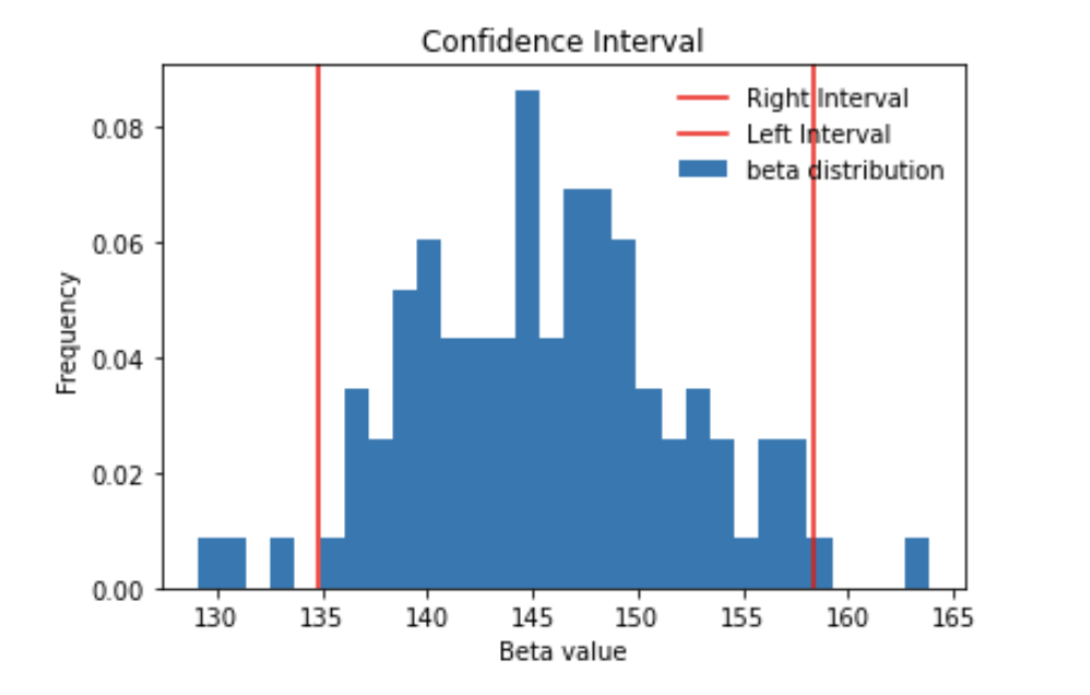
Use the helper code plot_simulation() to visualise the $\beta$ values along with its confidence interval

Hints¶

np.random.randint() : Returns list of integers as per mentioned size

df.iloc[] : Purely integer-location based indexing for selection by position

plt.hist() : Plots a histogram

plt.axvline() : Adds a vertical line across the axes

plt.axhline() : Add a horizontal line across the axes

plt.xlabel() : Sets the label for the x-axis

plt.ylabel() : Sets the label for the y-axis

plt.legend() : Place a legend on the axes

ndarray.sort() :Returns the sorted ndarray.

np.percentile(list, q) : Returns the q-th percentile value based on the provided ascending list of values.

Note: This exercise is auto-graded and you can try multiple attempts.

In [1]:

# import the libraries
import pandas as pd
import numpy as np
import matplotlib.pyplot as plt
%matplotlib inline

Reading the standard Advertising dataset¶

In [2]:

# Read the 'Advertising_adj.csv' file
df = pd.read_csv('Advertising_adj.csv')

In [7]:

# Use your bootstrap function from the previous exercise
def bootstrap(df):
    selectionIndex = np.random.randint(len(df), size = len(df))
    new_df = df.iloc[selectionIndex]
    return new_df

In [8]:

# Like last time, create a list of beta values using 1000 bootstraps of your original data
beta0_list, beta1_list = [],[]

numberOfBootstraps = 100

for i in range(numberOfBootstraps):
    df_new = bootstrap(df)
    
    xmean = df_new.tv.mean()
    ymean = df_new.sales.mean()
    
    beta1 = np.dot((df_new.tv-xmean) , (df_new.sales-ymean))/((df_new.tv-xmean)**2).sum()
    beta0 = ymean - beta1*xmean
    
    beta0_list.append(beta0)
    beta1_list.append(beta1)

In [9]:

### edTest(test_sort) ###

# Sort the two lists of beta values  from lowest value to highest 
beta0_list.___;
beta1_list.___;

In [10]:

### edTest(test_beta) ###

# Now we find the confidence interval
# Find the 95% percent confidence interval using the percentile function
beta0_CI = (np.___,np.___)

beta1_CI = (np.___,np.___)

In [ ]:

#Print the confidence interval of beta0 upto 3 decimal points
print(f'The beta0 confidence interval is {___}')

In [ ]:

#Print the confidence interval of beta1 upto 3 decimal points
print(f'The beta1 confidence interval is {___}')

In [15]:

# Use this helper function to plot the histogram of beta values along with the 95% confidence interval
def plot_simulation(simulation,confidence):
    plt.hist(simulation, bins = 30, label = 'beta distribution', align = 'left', density = True)
    plt.axvline(confidence[1], 0, 1, color = 'r', label = 'Right Interval')
    plt.axvline(confidence[0], 0, 1, color = 'red', label = 'Left Interval')
    plt.xlabel('Beta value')
    plt.ylabel('Frequency')
    plt.title('Confidence Interval')
    plt.legend(frameon = False, loc = 'upper right')

In [ ]:

# Plot for beta 0
plot_simulation(_,_)

In [ ]:

#Plot for beta 1
plot_simulation(_, _)