Key Word(s): model selection, cross validation
Instructions:
- Read the dataset and split into train and validation sets
- Select a max degree value for the polynomial model
- Fit a polynomial regression model for each degree to the training data and predict on the validation data
- Compute the train and validation error as MSE values and store in separate lists.
- Find out the best degree of the model.
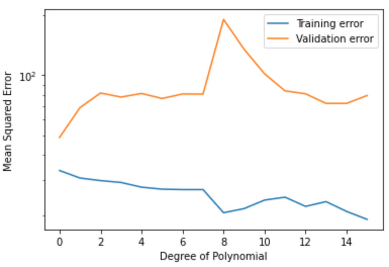
- Plot the train and validation errors for each degree.
Hints:
pd.read_csv(filename) : Returns a pandas dataframe containing the data and labels from the file data
sklearn.train_test_split() : Splits the data into random train and test subsets.
sklearn.PolynomialFeatures() : Generates a new feature matrix consisting of all polynomial combinations of the features with degree less than or equal to the specified degree
sklearn.fit_transform() : Fits transformer to X and y with optional parameters fit_params and returns a transformed version of X
sklearn.LinearRegression() : LinearRegression fits a linear model
sklearn.fit() : Fits the linear model to the training data
sklearn.predict() : Predict using the linear model.
plt.subplots() : Create a figure and a set of subplots
operator.itemgetter() : Return a callable object that fetches item from its operand
zip() : Makes an iterator that aggregates elements from each of the iterables.
Note: This exercise is auto-graded and you can try multiple attempts.
#import libraries
%matplotlib inline
import operator
import numpy as np
import pandas as pd
import matplotlib.pyplot as plt
from sklearn.model_selection import train_test_split
from sklearn.preprocessing import PolynomialFeatures
from sklearn.linear_model import LinearRegression
from sklearn.metrics import mean_squared_error
Reading the dataset
#Read the file "dataset.csv" as a dataframe

filename = "dataset.csv"

df = pd.read_csv(filename)
# Assign the values to the predictor and response variables

x = df[['x']].___
y = df.y.___
Train-validation split
### edTest(test_random) ###

#Split the dataset into train and validation sets with 75% Training set and 25% validation set.
#Set random_state=1

x_train, x_val, y_train, y_val = train_test_split(___)
Computing the train and validation error in terms of MSE
### edTest(test_regression) ###
# To iterate over the range, select the maximum degree of the polynomial
maxdeg = ___

# Create two empty lists to store training and validation MSEs
training_error, validation_error = [],[]

#Run a for loop through the degrees of the polynomial, fit linear regression, predict y values and calculate the training and testing errors and update it to the list
for d in range(maxdeg):

    #Compute the polynomial features for the train and validation sets
    x_poly_train = PolynomialFeatures(d).fit_transform(___)
    x_poly_val = PolynomialFeatures(d).fit_transform(___)

    lreg = LinearRegression()
    lreg.fit(x_poly_train, y_train)

    y_train_pred = lreg.predict(___)
    y_val_pred = lreg.predict(___)

    #Compute the train and validation MSE

    training_error.append(mean_squared_error(___))
    validation_error.append(mean_squared_error(___))
Finding the best degree
### edTest(test_best_degree) ###

#The best degree is the model with the lowest validation error

min_mse = min(validation_error)

best_degree = validation_error.index(min_mse)

print("The best degree of the model is",best_degree)
Plotting the error graph
# Plot the errors as a function of increasing d value to visualise the training and testing errors

fig, ax = plt.subplots()

#Plot the training error with labels

ax.plot(___)

#Plot the validation error with labels

ax.plot(___)

# Set the plot labels and legends

ax.set_xlabel('Degree of Polynomial')
ax.set_ylabel('Mean Squared Error')
ax.legend(loc = 'best')
ax.set_yscale('log')
plt.show()
Once you have marked your exercise, run again with Random_state = 0
Do you see any change in the results with change in the random state? If so, what do you think is the reason behind it?
Your answer here