Title¶

Exercise: A.2 - MSE for varying β1 values

Description¶

The goal here is to produce a plot like the one given below.

Instructions:¶

We want to find the model that fit best the data. To do so we are going to

1) Fix $\beta_0 = 2.2$,

2) Change $\beta_1$ in a range $[-2, 3]$, and

3) Estimate the fit of the model.

Create empty lists;

Set a range of values for $\beta_1$ and compute MSE for each one;

Compute MSE for varying $\beta_1$

Hints:¶

np.linspace(start, stop, num) : Return evenly spaced numbers over a specified interval.

np.arange(start, stop, increment) : Return evenly spaced values within a given interval

list_name.append(item) : Add an item to the end of the list

plt.xlabel() : This is used to specify the text to be displayed as the label for the x-axis

plt.ylabel() : This is used to specify the text to be displayed as the label for the y-axis

Note: This exercise is auto-graded and you can try multiple attempts

In [13]:

import numpy as np
import pandas as pd
import matplotlib.pyplot as plt
%matplotlib inline

Reading the dataset¶

In [14]:

# Data set used in this exercise 
data_filename = 'Advertising.csv'

# Read data file using pandas libraries
df = pd.read_csv(data_filename)

In [16]:

# Take a quick look at the data
df.head()

Out[16]:

	TV	Radio	Newspaper	sales
0	230.1	37.8	69.2	22.1
1	44.5	39.3	45.1	10.4
2	17.2	45.9	69.3	9.3
3	151.5	41.3	58.5	18.5
4	180.8	10.8	58.4	12.9

In [17]:

# Create a new dataframe called `df_new`. witch the columns ['TV' and 'sales'].
df_new = df[['TV', 'sales']]

Beta and MSE Computation¶

In [6]:

# Set beta0 
beta0 = 2.2

In [12]:

# Create lists to store the MSE and beta1
mse_list = ___
beta1_list = ___

In [ ]:

### edTest(test_beta) ###

# This loops runs from -2 to 3.0 with an increment of 0.1 i.e a total of 51 steps
for beta1 in ___:
    
    # Calculate prediction of x using beta0 and beta1
    y_predict = ___ 
    
    # Calculate Mean Squared Error
    mean_squared_error = ___

    # Append the new MSE in the list that you created above
    mse_list.___ 
    
    # Also append beta1 values in the list
    beta1_list.___

Plotting the graph¶

In [ ]:

### edTest(test_mse) ###
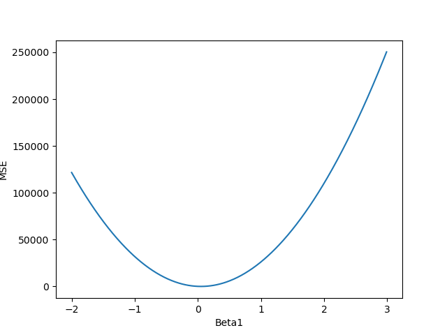
# Plot MSE as a function of beta1
plt.plot(beta1_list, mse_list)
plt.xlabel('Beta1')
plt.ylabel('MSE')

Go back and change your $\beta_0$ value and report your new optimal $\beta_1$ value and new lowest $MSE$¶

Is the MSE lower than before, or more?

In [ ]:

# Your answer here