 CS109A Introduction to Data Science
Lecture 4, Exercise 2: EDA and Advanced PANDAS
Harvard University
Fall 2020
Instructors: Pavlos Protopapas, Kevin Rader, and Chris Tanner
import pandas as pd
import seaborn as sns
pd.set_option('display.width', 500)
pd.set_option('display.max_columns', 100)
NOTE: After running every cell, be sure to auto-grade your work by clicking 'Mark' in the lower-right corner. Otherwise, no credit will be given.
Advanced PANDAS
We will use the same top50.csv file from Exercise 1.
Below, fill in the blank to create a new PANDAS DataFrame from the top50.csv file.
### edTest(test_a) ###
df = _____
Run the cell below to print the summary statistics and display the column names
print(df.columns)
df.describe()
Fill in the blank to set longest_song equal to the TrackName of the longest song (the song that has the highest Length value)
### edTest(test_b) ###
longest_song = __________
longest_song
Fill in the blank to set loud_song equal to the TrackName of the song that has the highest Loudness value amongst the 10 most popular songs. To be clear, by highest we mean the least negative. So, we would say that -2 is louder than -10.
### edTest(test_c) ###
loud_song = _______________
loud_song
Say you are interested in songs that last 3-4 minutes, anything shorter doesn't have time to build up a narrative, and anything longer gets boring. You have a very particular taste but are open to listening to what other people are listening to a lot, but you don't even know what genre that is!
Fill in the blank below (or use multiple lines if you prefer) to set new_genre to be the genre that is associated with the most songs that are between 3 and 4 minutes in duration (including songs that are exactly 3 minutes and 4 minutes).
### edTest(test_d) ###
new_genre = ____________________
new_genre
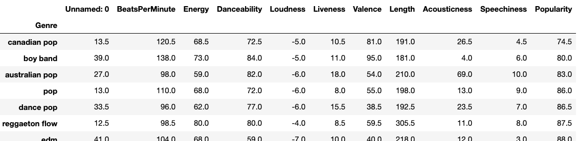
Below, fill in the blank to make a new DataFrame genre_counts that groups all songs by their Genre and aggregates all other columns by their median value. Then, sort by their Popularity (in ascending order).
As an example, if df had only 3 "pop" songs, and their Danceability values were 70,82, and 90, and df also contained 5 "latin" songs, and their Danceability values were 80,82,90,91,99. Then genre_counts would have 1 row for the Genre "pop", with a Danceability value of 82. genre_counts would also have 1 row for the Genre "latin", with a Danceability value of 90. Then, we'd sort the DataFrame by the Popularity (in ascending order).
For example, your DataFrame should look as follows (snippet):
### edTest(test_e) ###
new_df = _______________
new_df
Below, fill in the blank to set the variable speechy_song to the TrackName of the song that has the highest Speechiness value
### edTest(test_f) ###
speechy_song = _______________
speechy_song
END OF GRADED SECTION
EXTRA EXAMPLES FOLLOW:
Combining multiple DataFrames
As mentioned, often times one dataset doesn't contain all of the information you are interested in -- in which case, you need to combine data from multiple files. This also means you need to verify the accuracy (per above) of each dataset.
spotify_aux.csv contains the same 50 songs as top50.csv; however, it only contains 3 columns:
- Track Name
- Artist Name
- Explicit Language (boolean valued)
Note, that 3rd column is just random Boolean values, but pretend as if it's correct. The point of this section is to demonstrate how to merge columns together.
Let's load spotify_aux.csv into a DataFrame:
explicit_lyrics = pd.read_csv("spotify_aux.csv")
explicit_lyrics
Let's merge it with our df DataFrame that is storing top50.csv.
.merge() is a Pandas function that stitches together DataFrames by their columns.
.concat() is a Pandas function that stitches together DataFrames by their rows (if you pass axis=1 as a flag, it will be column-based)
# 'on='' specifies the column used as the shared key
df_combined = pd.merge(explicit_lyrics, df, on='TrackName')
df_combined
We see that all columns from both DataFrames have been added. That's nice, but having duplicate ArtistName and TrackName is unecessary. Since merge() uses DataFrames as the passed-in objects, we can simply pass merge() a stripped-down copy of ExplicitLanguage, which helps merge() not add any redundant fields.
df_combined2 = pd.merge(explicit_lyrics[['TrackName', 'ExplicitLanguage']], df, on='TrackName')
df_combined2
You'll notice we don't have the same number of rows as our original df DataFrame.
Why is that? What happened? How can we quickly identify which rows are missing -- especially if our dataset had thousands of rows. Discuss with your group.
Related to merge, are the useful functions:
concat()aggregate()append()
Plotting DataFrames
As a very simple example of how one can plot elements of a DataFrame, we turn to Pandas' built-in plotting:
scatter_plot = df.plot.scatter(x='Danceability', y='Popularity', c='DarkBlue')
scatter_plot

This shows the lack of a correlation between the Danceability of a song and its popularity, based on just the top 50 songs, of course.
Please feel free to experiment with plotting other items of interest.
Print the songs that are faster than the average Top 50 and more popular than the average Top 50?
avg_speed = df['BeatsPerMinute'].mean()
avg_popularity = df['Popularity'].mean()
df[(df['BeatsPerMinute'] > avg_speed) & (df['Popularity'] > avg_popularity)]