Lecture 20¶

Tuesday, November 12th 2019¶

Dynamic Arrays, Python Internals, I/O¶

Note: Please download this notebook.¶

Certain cells cannot render on the website.

Last time:¶

• Generators
• How generators work
• Start on Python internals

This time:¶

• Dynamic arrays
• How things work
• Overview of some I/O

In Python you can append to lists. So what's an ob_size doing in our struct then?

typedef struct {
    long ob_refcnt;
    PyTypeObject *ob_type;
    Py_ssize_t ob_size;
    PyObject **ob_item;
    long allocated;
} PyListObject;

Turns out Python lists are implemented in something called a dynamic array.

Big O Notation¶

• Part of a larger notion of limiting behavior of functions
  • Including Small O, Big Theta, Big Omega, Small Omega

• For us, it just means "bounded above"

• More strictly: $$f\left(n\right) = \mathcal{O}\left(g\left(n\right)\right)$$ means $\left|f\right|$ is bounded above by $g$ asymptotically.

Example: Binary Search Trees¶

• We have stated that the time-complexity of BSTs is $\mathcal{O}\left(\log\left(n\right)\right)$

• This means that the time-complexity is bounded above by $\log\left(n\right)$.

A complete binary tree has $$n = 1 + 2 + \ldots + 2^{h-1} + 2^{h}$$ nodes where $h$ is the height of the tree.

We can write this as $$n=2^{h+1} - 1.$$

Solving for the height gives $$h = \log_{2}\left(n+1\right) - 1.$$

So the height scales like $\log_{2}\left(n\right)$.

Going just a little bit further we have \begin{align*} h &= \log_{2}\left(n+1\right) - 1 \\ & < \log_{2}\left(n+1\right). \end{align*}

So the height is bounded from above by $\log_{2}\left(n+1\right)$.

But asymptotically, as $n\to\infty$, $\log_{2}\left(n+1\right)$ behaves like $\log_{2}\left(n\right)$.

Arrays¶

A static array is a contiguous slab of memory of known size, such that n items can fit in. This is a great data structure. Why?

• constant time index access: a[i] is $\mathcal{O}(1)$
  • Just go directly to i * sizeof(int)

• linear time traversal or search: $1$ unit / loop iteration means $\mathcal{O}(n)$ in loop.

• locality in memory: it's one int after another

Tuples in Python are fixed size, static arrays.

But the big problem is, what if we want to add something more beyond the end of the array?

Then we must use dynamic arrays.

Note that this shifts the focus more to space complexity (rather than time complexity).

Dynamic Arrays¶

What Python does is first create a fixed size array of these PyListObject* pointers on the heap. Then, as you append, it uses its own algorithm to figure out when to expand the size of the array.

listobject.c

/* This over-allocates proportional to the list size, making
 * room for additional growth.  The over-allocation is mild, 
 * but is enough to give linear-time amortized behavior over a 
 * long sequence of appends() in the presence of a poorly- 
 * performing system realloc().  The growth pattern is:  0, 4, 
 * 8, 16, 25, 35, 46, 58, 72, 88, ...
*/
new_allocated = (newsize >> 3) + (newsize < 9 ? 3 : 6);

An empty list is 64 bytes.

Each int adds an 8 byte pointer.

Note: The growth factor is less than $2$! This is quite technical, but here is a reference: https://en.wikipedia.org/wiki/Dynamic_array#Growth_factor.

Performance of Dynamic Arrays¶

Let's assume we start with an array of size of $1$ (one slot) and then double the size each time. After $n$ doublings, we have an array with $2^n$ slots. So, it then takes $\log(n)$ doublings for the array to have $n$ slots (note, $\log(n)$ means $\log_{2}(n)$).

Notice that we might not get the continuously allocated memory we want. So we'll have to recopy to a larger array.

The last $n/2$ numbers in the array don't move at all (they're the new ones). The previous $n/4$ numbers in the array would have moved once, the previous $n/8$ twice, and so on.

Therefore, the $i$-th chunk of numbers will have moved $$i \dfrac{n}{2^{i+1}}$$ times. Show this!!

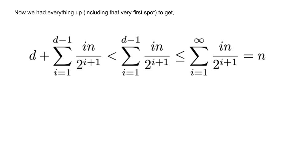
We need to add all these movements up.

Thus the total number of movements is

This is an amazing result. The work of reallocation is still $\mathcal{O}(n)$ on the average, as if a single array had been allocated in advance!

Here's the calculation.

When $x = 1/2$ we have $$\sum_{i=0}^{\infty}{\left(i+1\right)x^{i+1}} = 2.$$ So, to summarize, $$\dfrac{n}{2}\sum_{i=1}^{\infty}{\dfrac{i}{2^{i}}} = \dfrac{n}{2}\sum_{i=0}^{\infty}{\dfrac{i+1}{2^{i+1}}} = \dfrac{n}{2}\times 2 = n.$$

Containers vs Flats¶

Earlier we saw how Python lists contained references to integer ("digit")+metdata based structs on the heap.

We call sequences that hold such "references" to objects on the heap Container Sequences. Examples of such container sequences are list, tuple, collections.deque.

There are collections in Python which contain contiguous "typed" memory (which itself is allocated on the heap). We call these Flat Sequences. Such containers in Python 3 are: str, bytes, bytearray, memoryview, array.array.

You have probably extensively used a type of flat sequence not mentioned yet. This is NumPy's ndarray: np.array.

All of these are faster as they work with contiguous blocks of uniformly formatted memory.

From Fluent Python:

Container sequences hold references to the objects they contain, which may be of any type, while flat sequences physically store the value of each item within its own memory space, and not as distinct objects. Thus, flat sequences are more compact, but they are limited to holding primitive values like characters, bytes, and numbers.

The data structures we have discussed fall into two general classes:

Contiguously-allocated structures are composed of single slabs of memory, and include arrays, matrices, heaps, and hash tables. These are the Flat Sequences we described above.

Linked data structures are composed of independent chunks of memory bound together by pointers, and include lists, trees, and graph adjacency lists. These are the Container Sequences we described above.

(Steven S Skiena. The Algorithm Design Manual)

• A critical advantage of something like a contiguous memory array is that indexing is a constant time operation, as opposed to worst-case $\mathcal{O}(n)$, as we saw in linked lists.
• Other benefits include a tighter size and a locality of memory which benefits cache and general memory transport.

Mutable vs Immutable¶

The mutability of objects has recurred often in this course.

One can also study containers based on their mutability.

Mutable sequences in Python 3 are: list, bytearray, array.array, collections.deque, memoryview.

Immutable sequences in Python 3 are tuple, str, bytes.

Let's learn about some of these collections in Python.

array.array¶

The list type is nice and very flexible, but if you need to store many many (millions) of floating point variables, array.array is a better option.

array.array stores just the bytes representing the type, so its just like a contiguous C array of things in RAM, and also just like a numpy array.

array.array is mutable, and you don't need to allocate ahead of time (reallocation will be done).

Now let's do the same thing with a list comprehension:

A Few Observations¶

• Looks like a regular Python list on a billion floats only costs double (seems like it should be even slower...).
• Why is accessing floats in an array.array so slow?
  • Because each float is boxed by the Python runtime. You saw this earlier!

In an array.array or in numpy.array for that matter, when you "iterate" over the array, and use the ints you get, what Python does is to take that 32 bits or 64 bits from memory, wrap it up into one of these structs, and hand it to you. You asked for a Python int after all.

Operations on array.array which can be done with C are fast; access into Python is slow.

This is why numpy.ndarray is written in C, with operations like numpy.dot written in C.

(None of the array.array functionality is exposed with any complex operations under the hood, so its current use remains limited.)

If you want to use numerical stuff, use numpy arrays.

See https://www.python.org/doc/essays/list2str/ for a discussion on when it's a good idea to use array.array.

memoryviews¶

Memoryviews, inspired by NumPy and SciPy, let you handle slices of arrays without expensively copying bytes.

Travis Oliphant, as quoted in Fluent:

A memoryview is essentially a generalized NumPy array structure in Python itself (without the math). It allows you to share memory between data-structures (things like PIL images, SQLlite databases, NumPy arrays, etc.) without first copying. This is very important for large data sets.

Additional Details on Dynamic Arrays¶

The cartoons below are meant to help you see how to count the number of movements. The variable $d$ reperesents the number of doublings.

Doublings¶

After $4$ doublings, the array looks something like, 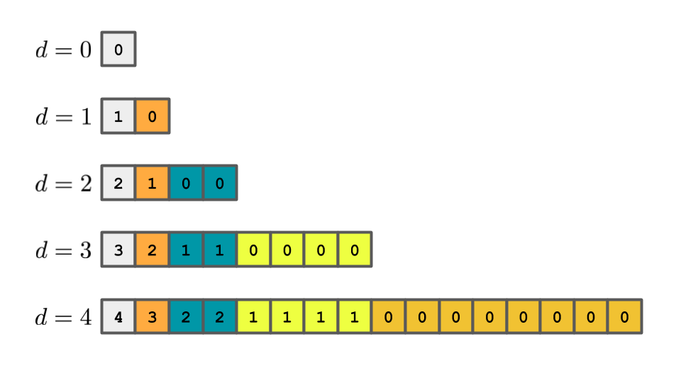The numbers in each cell represent the number of times that cell was moved (or copied). These numbers are not the numbers in the array.

By the time the fourth doubling occurs, the first cell has been copied $4$ times, the next cell has been copied $3$ times, the next $2$ cells have been copied $2$ times each and so on.

Bookkeeping¶

The figure below shows how you might count the number of movements in each chunk. None of the cells in the most recent chunk have been moved yet. Each cell in the second-most recent chunk have been copied one time, which corresponds to $4$ total movements in that chunk. This same pattern can be observed in all the chunks.

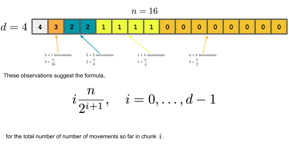
Note that the very first chunk has been copied $d$ times (the number of doublings).

Addition¶

Now we simply add all of these movements up. The first chunk has moved $d$ times, the second chunk has moved $d-1\times\dfrac{n}{2^{d}}$ times, etc. The final result is illustrated in the figure below.

I/O Intro¶

• Input Files
  • XML
  • YAML
  • JSON
• Comments on pickling

Input Files and Parsing¶

We usually want to read data into our software:

• Input parameters to the code (e.g. time step, linear algebra solvers, physical parameters, etc)
• Input fields (e.g. fields to visualize)
• Calibration data
• $\vdots$

This data can be provided by us, or the client, or come from a database somewhere.

There are many ways of reading in and parsing data. In fact, this is often a non-trivial exercise depending on the quality of the data as well as its size.

XML Intro¶

What is XML?¶

Note: Material presented here taken from the following sources

• https://www.w3schools.com/xml/default.asp
• https://docs.python.org/2/library/xml.etree.elementtree.html
• https://www.w3.org/TR/2008/REC-xml-20081126/
• https://en.wikipedia.org/wiki/XML

Some basic XML comments:

• XML stands for Extensible Markup Language
• XML is just information wrapped in tags
• It doesn't do anything per se
• Its format is both machine- and human-readable

Some Basic XML Anatomy¶

 

 
     id="dog1"> 
         Cloe  
         3  
         Border Collie 
         Yes 
    
     id="dog2"> 
         Karl  
         7 
         Beagle 
         Yes 
    

Note that all XML elements have a closing tag!

Some More Basic XML Anatomy¶

See w3schools XML tutorial for a very nice summary of the essential XML rules.

XML elements: a few things to be aware of:

• Elements can contain text, attributes, and other elements
• XML names are case sensitive and cannot contain spaces
• Be consistent in your naming convention

XML attributes: a few things to be aware of:

• XML attributes must be in quotes
• There are no rules about when to use elements or attributes
  • You could make an attribute an element and it might read better
• Rule of thumb: Data should be stored as elements. Metadata should be stored as attributes.

Python and XML¶

We will use the ElementTree class to read in and parse XML input files in Python.

A very nice tutorial can be found in the Python ElementTree documentation.

We'll work with the shelterdogs.xml file to start.

Looping Over Child Elements¶

Accessing Children by Index¶

The Element.iter() Method¶

From the documentation:

Creates a tree iterator with the current element as the root. The iterator iterates over this element and all elements below it, in document (depth first) order.

The Element.findall() Method¶

From the documentation:

Finds all matching subelements, by tag name or path. Returns a list containing all matching elements in document order.

What is JSON?¶

• Stands for JavaScript Object Notation
• It's actually language agnostic
  • No need to learn JavaScript to use it
• Like XML, it's a human-readable format

Some Basic JSON Anatomy¶

{
    "dogShelter": "MSPCA-Angell",
    "dogs": [
        {
            "name": "Cloe",
            "age": 3,
            "breed": "Border Collie",
            "attendPlaygroup": "Yes"
        },
        {
            "name": "Karl",
            "age": 7,
            "breed": "Beagle",
            "attendPlaygroup": "Yes"
        }
    ]
}

JSON and Python¶

• Python supports JSON natively
• Saving Python data to JSON format is called serialization
• Loading a JSON file into Python data is called deserialization

Deserialization¶

Since we're interested in reading in some fancy input file, we'll begin by discussing deserialization.

We'll work with the shelterdogs.json file.

Comments on Deserialization¶

That was pretty nice! We got a Python dictionary out. We sure know how to work with Python dictionaries.

Serialization¶

You can also write data out to JSON format. Let's just do a brief example.

Some JSON References¶

• www.json.org
• Wikipedia page
• Working with JSON data in Python
• w3schools JSON syntax

What is YAML?¶

• The official website: YAML
• From the official website:
  • YAML stands for YAML Ain't Markup Language
    • Example of a recursive acronym (like Linux!)
  • "What It Is: YAML is a human-friendly data serialization standard for all programming languages."
• YAML is quite friendly to use and continues to gain in popularity

YAML Anatomy¶

shelterDogs:
- {age: 3, attendPlaygroup: 'Yes', breed: Border Collie, name: Cloe}
- {age: 7, attendPlaygroup: 'Yes', breed: Beagle, name: Karl}
shelterStaff:
- {Job: dogWalker, age: 100, name: Bob}
- {Job: PlaygroupLeader, age: 47, name: Sally}

Serialization¶

Deserialization¶

What is pickle?¶

• Python has it's own module for loading and writing python data
• Part of the python standard library
• Fast
• Can store arbitrarily complex Python data structures

Some caveats¶

• Python specific: no guarantee of cross-language compatibility
• Not every python datastructure can be serialized by pickle
• Older versions of python don't support newer serialization formats
  • Lastest format can handle the most python datastructures
  • They can also read in older datastructures
  • Older formats cannot read in newer formats
• Make sure to use binary mode when opening pickle files
  • Data will get corrupted otherwise