References
- A Hitchhiker’s Guide to Automatic Differentiation
- Griewank, A. and Walther, A., 2008. Evaluating derivatives: principles and techniques of algorithmic differentiation (Vol. 105). Siam.
- Nocedal, J. and Wright, S., 2001. Numerical Optimization, Second Edition. Springer.
- Automatic Differentiation in Machine Learning: A Survey
Today
- Towards the reverse mode
Towards the Reverse Mode
The focus of this class is on the forward mode of automatic differentiation. The reverse mode is also extremely popular and useful (e.g. in scenarios that have $f:\mathbb{R}^{m}\mapsto\mathbb{R}$). Here we will outline the mechanics of the reverse mode, show a little example, and survey the basic equations.
A Sketch of the Reverse Mode
- Create evaluation graph
- Forward pass does function evaluations
- Forward pass also does partial derivatives of elementary functions
- It does NOT do the chain rule!
- Just stores the partial derivatives
- If $x_{3} = x_{1}x_{2}$ is a node, we store $\dfrac{\partial x_{3}}{\partial x_{1}}$ and $\dfrac{\partial x_{3}}{\partial x_{2}}$. That's it.
- Reverse pass starts with $\overline{x}_{N} = \dfrac{\partial f}{\partial x_{N}} = 1$ (since $f$ is $x_{N}$)
- Then it gets $\overline{x}_{N-1} = \dfrac{\partial f}{\partial x_{N}}\dfrac{\partial x_{N}}{\partial x_{N-1}}$
- Note: $\dfrac{\partial x_{N}}{\partial x_{N-1}}$ is already stored from the forward pass
- The only trick occurrs when we get to a branch in the graph. That is, when the node we're on has more than one child. In that case, we sum the two paths. For example, if $x_{3}$ has $x_{4}$ and $x_{5}$ as children, then we do $$\overline{x}_{3} = \dfrac{\partial f}{\partial x_{3}} = \dfrac{\partial f}{\partial x_{4}}\dfrac{\partial x_{4}}{\partial x_{3}} + \dfrac{\partial f}{\partial x_{5}}\dfrac{\partial x_{5}}{\partial x_{3}}.$$
- Note: This summation is a manifestation of the chain rule.
The reverse mode cannot be interpreted in the context of dual numbers like the forward mode was.
The little implementation sketch that we did for the forward mode will need to be generalized for the reverse mode.
The Basic Equations
These equations are modified from Nocedal and Wright (page 180).
The partial derivative of $f$ with respect to $x_{i}$ can be written as \begin{align} \dfrac{\partial f}{\partial x_{i}} = \sum_{\text{j a child of i}}{\dfrac{\partial f}{\partial x_{j}}\dfrac{\partial x_{j}}{\partial x_{i}}}. \end{align} At each node $i$ we compute \begin{align} \overline{x}_{i} += \dfrac{\partial f}{\partial x_{j}}\dfrac{\partial x_{j}}{\partial x_{i}}. \end{align} The $\overline{x}_{i}$ variable stores the current value of the partial derivative at node $i$. It is sometimes called the adjoint variable.
An Example for Intuition
Let's try to evaluate the function $$f\left(x,y\right) = xy + \exp\left(xy\right)$$ and its gradient at the point $a = (1,2)$. We'll use the reverse mode this time.
Clearly we have $$\nabla f = \begin{bmatrix} y + \exp\left(xy\right)y \\ x + \exp\left(xy\right)x \end{bmatrix}.$$ Hence \begin{align} f\left(a\right) &= 2 + e^{2} \\ \nabla f &= \begin{bmatrix} 2 + 2e^{2} \\ 1 + e^{2} \end{bmatrix}. \end{align}
Here's a visualization of the computational graph:
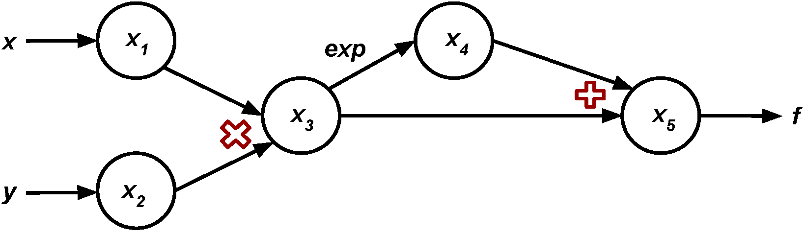
Let's use the reverse mode to calculate the gradient of $f$.
- Generate the forward trace and calculate the partial derivatives of a node wrt its children.
- Notice that this time we need to save the graph.
- Start at $x_{5}$ and start calculating the chain rule.
| Node | Current Value | Numerical Value | $\partial_{1}$ | $\partial_{1}$ Value | $\partial_{2}$ | $\partial_{2}$ Value |
|---|---|---|---|---|---|---|
| $x_{1}$ | $x$ | $1$ | $1$ | $1$ | $0$ | $0$ |
| $x_{2}$ | $y$ | $2$ | $0$ | $0$ | $1$ | $1$ |
| $x_{3}$ | $x_{1}x_{2}$ | $2$ | $x_{2}$ | $2$ | $x_{1}$ | $1$ |
| $x_{4}$ | $\exp\left(x_{3}\right)$ | $e^{2}$ | $\exp\left(x_{3}\right)$ | $e^{2}$ | $-$ | $-$ |
| $x_{5}$ | $x_{3} + x_{4}$ | $2 + e^{2}$ | $1$ | $1$ | $1$ | $1$ |
$\overline{x}_{5} = \dfrac{\partial f}{\partial x_{5}} = 1$
| Node | Current Value | Numerical Value | $\partial_{1}$ | $\partial_{1}$ Value | $\partial_{2}$ | $\partial_{2}$ Value |
|---|---|---|---|---|---|---|
| $x_{1}$ | $x$ | $1$ | $1$ | $1$ | $0$ | $0$ |
| $x_{2}$ | $y$ | $2$ | $0$ | $0$ | $1$ | $1$ |
| $x_{3}$ | $x_{1}x_{2}$ | $2$ | $x_{2}$ | $2$ | $x_{1}$ | $1$ |
| $x_{4}$ | $\exp\left(x_{3}\right)$ | $e^{2}$ | $\exp\left(x_{3}\right)$ | $e^{2}$ | $-$ | $-$ |
| $x_{5}$ | $x_{3} + x_{4}$ | $2 + e^{2}$ | $1$ | $1$ | $1$ | $1$ |
$\overline{x}_{4} = \dfrac{\partial f}{\partial x_{5}}\dfrac{\partial x_{5}}{\partial x_{4}} = 1 \cdot 1 = 1$
| Node | Current Value | Numerical Value | $\partial_{1}$ | $\partial_{1}$ Value | $\partial_{2}$ | $\partial_{2}$ Value |
|---|---|---|---|---|---|---|
| $x_{1}$ | $x$ | $1$ | $1$ | $1$ | $0$ | $0$ |
| $x_{2}$ | $y$ | $2$ | $0$ | $0$ | $1$ | $1$ |
| $x_{3}$ | $x_{1}x_{2}$ | $2$ | $x_{2}$ | $2$ | $x_{1}$ | $1$ |
| $x_{4}$ | $\exp\left(x_{3}\right)$ | $e^{2}$ | $\exp\left(x_{3}\right)$ | $e^{2}$ | $-$ | $-$ |
| $x_{5}$ | $x_{3} + x_{4}$ | $2 + e^{2}$ | $1$ | $1$ | $1$ | $1$ |
$\overline{x}_{3} = \dfrac{\partial f}{\partial x_{4}}\dfrac{\partial x_{4}}{\partial x_{3}} + \dfrac{\partial f}{\partial x_{5}}\dfrac{\partial x_{5}}{\partial x_{3}}= 1 \cdot e^{2} + 1\cdot 1 = 1 + e^{2}$
| Node | Current Value | Numerical Value | $\partial_{1}$ | $\partial_{1}$ Value | $\partial_{2}$ | $\partial_{2}$ Value |
|---|---|---|---|---|---|---|
| $x_{1}$ | $x$ | $1$ | $1$ | $1$ | $0$ | $0$ |
| $x_{2}$ | $y$ | $2$ | $0$ | $0$ | $1$ | $1$ |
| $x_{3}$ | $x_{1}x_{2}$ | $2$ | $x_{2}$ | $2$ | $x_{1}$ | $1$ |
| $x_{4}$ | $\exp\left(x_{3}\right)$ | $e^{2}$ | $\exp\left(x_{3}\right)$ | $e^{2}$ | $-$ | $-$ |
| $x_{5}$ | $x_{3} + x_{4}$ | $2 + e^{2}$ | $1$ | $1$ | $1$ | $1$ |
$\overline{x}_{2} = \dfrac{\partial f}{\partial x_{3}}\dfrac{\partial x_{3}}{\partial x_{2}} = \left(1 + e^{2}\right)x_{1} = 1 + e^{2} = \dfrac{\partial f}{\partial y}$
| Node | Current Value | Numerical Value | $\partial_{1}$ | $\partial_{1}$ Value | $\partial_{2}$ | $\partial_{2}$ Value |
|---|---|---|---|---|---|---|
| $x_{1}$ | $x$ | $1$ | $1$ | $1$ | $0$ | $0$ |
| $x_{2}$ | $y$ | $2$ | $0$ | $0$ | $1$ | $1$ |
| $x_{3}$ | $x_{1}x_{2}$ | $2$ | $x_{2}$ | $2$ | $x_{1}$ | $1$ |
| $x_{4}$ | $\exp\left(x_{3}\right)$ | $e^{2}$ | $\exp\left(x_{3}\right)$ | $e^{2}$ | $-$ | $-$ |
| $x_{5}$ | $x_{3} + x_{4}$ | $2 + e^{2}$ | $1$ | $1$ | $1$ | $1$ |
$\overline{x}_{1} = \dfrac{\partial f}{\partial x_{3}}\dfrac{\partial x_{3}}{\partial x_{1}} = \left(1 + e^{2}\right)x_{2} = 2 + 2e^{2} = \dfrac{\partial f}{\partial x}$
Exercise 1
Consider the function $$f\left(w_{1}, w_{2}, w_{3}, w_{4}, w_{5}\right) = w_{1}w_{2}w_{3}w_{4}w_{5}$$ evaluated at the point $a = \left(2, 1, 1, 1, 1\right)$.
- Calculate the gradient using the reverse mode.
- You may want to start by drawing the graph to help you visualize.
- Set up an evaluation table. Note that this table can have the same columns as the example in class.
- Write out the reverse mode based on the evaluation table.
- Calculate the gradient using forward mode.
- You can use the same graph as in the reverse mode.
- Set up a forward evaluation table. Note that this table will have more columns than the one you created for the reverse mode.
- For both forward and reverse mode, calculate the number of operations.
- Hint: You may count only the floating point operations (e.g. addition and multiplication). You are not required to count memory access steps, retrievals, etc.
Observations
- The forward and reverse modes give the same answer.
- Forward mode calculation depends on number of independent variables
- Note: In many applications, a function will depend on some independent variables and be parameterized by some other variables (e.g. $L\left(x;\theta\right)$.
- In many optimization problems, we treat $\theta$ as the independent variable. It is a matter of perspective.
- The reverse mode calculation does not depend on the number of independent variables.
What Reverse Mode Actually Computes
- Recall that the forward mode actually computes the Jacobian-vector product $$Jp.$$
- We noted that the full Jacobian could be computed by choosing $m$ seed vectors where $m$ is the number of independent variables, independent of $n$, the number of functions.
What Reverse Mode Actually Computes
- The reverse mode computes $$J^{T}p$$ where $J^{T}$ is the transpose of the Jacobian.
- If you want the transpose of the Jacobian, this can be accomplished independent of the number of independent variables.
Connection to Backpropagation
- Backpropagation is a special case of the reverse mode of automatic differentiation.
- The special case is:
- The objective function is a scalar function.
- The objective function represents an error between the output and a true value.
Some Take-Aways
- Automatic differentiation can be used to compute derivatives to machine precision of functions $f:\mathbb{R}^{m} \to \mathbb{R}^{n}$.
Some Take-Aways
- Forward mode is more efficient when $n\gg m$.
- This corresponds to the case where the number of functions to evaluate is much greater than the number of inputs.
- Actually computes the Jacobian-vector product $Jp$.
Some Take-Aways
- Reverse mode is more efficient when $n\ll m$.
- This corresponds to the case where the number of inputs is much greater than the number of functions.
- Actually computes the Jacobian-transpose-vector product $J^{T}p$.
Some Take-Aways
- Backpropagation is a special case of the reverse mode applied to scalar objective functions.
Applications and Extensions
So far, you've seen the mechanics of AD and the key concepts.
But there are many extensions and applications.
We will discuss just a few.
Extensions
- Higher order derivatives and mixed derivatives.
- e.g. $\nabla\nabla f$, $\dfrac{\partial^{2} f}{\partial x^{2}}$, $\dfrac{\partial^{2} f}{\partial x \partial y}$, etc.
- Hessians and beyond
- Efficient computation
- Smart graph storage (if possible)
- Writing parts of the graph to disk and hold others in memory
- Combining forward and reverse mode
- Exploiting sparsity in the Jacobian and/or Hessian
- Non-differentiable functions
- Differential programming
Applications
There are a huge number of applications for AD. Here is a sampling of a few.
Numerical Solution of Ordinary Differential Equations
- Numerical integration of "stiff" differential equations.
- This is usually accomplished using implicit discretization methods (e.g. Backward Euler).
- Implicit methods require the solution of a nonlinear system of equations.
- This system can be solved with Newton's method.
- Newton's method requires Jacobian-vector products.
Optimization of Objective Functions
- Optimize an objective (a.k.a. loss, a.k.a. cost) function.
- This means to tune a set of parameters.
- Algorithms to accomplish this require derivatives of the ojective wrt the parameters.
- There are many types of objective functions out there.
Solution of Linear Systems
- Many problems reduce to the solution of a linear system $Ax = b$.
- Iterative methods are powerful algorithms for solving such problems.
- Some iterative methods require derivative information (e.g. steepest decent, conjugate gradient, biconjugate gradient, etc.)