Key Word(s): Automatic differentiation, Forward mode
References
- A Hitchhiker’s Guide to Automatic Differentiation
- Griewank, A. and Walther, A., 2008. Evaluating derivatives: principles and techniques of algorithmic differentiation (Vol. 105). Siam.
- Nocedal, J. and Wright, S., 2001. Numerical Optimization, Second Edition. Springer.
# Load libraries that we'll need
import matplotlib.pyplot as plt
import numpy as np
%matplotlib notebook
# or inline

def f(x):
    # Hard-coded f(x)
    return x - np.exp(-2.0 * np.sin(4.0*x) * np.sin(4.0*x))

def dfdx(x):
    # Hard-coded "Jacobian matrix" of f(x)
    return 1.0 + 16.0 * np.exp(-2.0 * np.sin(4.0*x) * np.sin(4.0*x)) * np.sin(4.0*x) * np.cos(4.0*x)

def dfdx_h(x, epsilon):
    return (f(x + epsilon) - f(x)) / epsilon
Introduction and Motivation
Differentiation is one of the most important operations in science. Finding extrema of functions and determining zeros of functions are central to optimization. Numerically solving differential equations forms a cornerstone of modern science and engineering and is intimately linked with predictive science.
Recap
Last time:
- Provided introduction and motivation for automatic differentiation (AD)
- Root-finding (Newton's method)
- The Jacobian
- The finite difference method
Today
- The basics of AD
- The computational graph
- Evaluation trace
- Computing derivatives of a function of one variable using the forward mode
- Computing derivatives of a function of two variables using the forward mode
- Just beyond the basics
- The Jacobian in forward mode
- What the forward mode actually computes
- Dual numbers
- Towards implementation
Note on Exercises
Today's exercises are mainly on pencil and paper. You do not need to turn these in.
Automatic Differentiation: The Mechanics and Basic Ideas
In the introduction, we motivated the need for computational techniques to compute derivatives. The focus in the introduction was on the finite difference method, but we also computed a symbolic derivative. The finite difference approach is nice because it is quick and easy. However, it suffers from accuracy and stability problems. On the other hand, symbolic derivatives can be evaluated to machine precision, but can be costly to evaluate. We'll have more to say about cost of symbolic differentiation later.
Automatic differentiation (AD) overcomes both of these deficiencies. It is less costly than symbolic differentiation while evaluating derivatives to machine precision. There are two modes of automatic differentiation: forward and reverse. This course will be primarily concerned with the forward mode. Time-permitting, we will give an introduction to the reverse mode. In fact, the famous backpropagation algorithm from machine learning is a special case of the reverse mode of automatic differentiation.
Review of the Chain Rule
At the heart of AD is the famous chain rule from calculus.
Back to the Beginning
Suppose we have a function $h\left(u\left(t\right)\right)$ and we want the derivative of $h$ with respect to $t$. The derivative is $$\dfrac{\partial h}{\partial t} = \dfrac{\partial h}{\partial u}\dfrac{\partial u}{\partial t}.$$ This is the rule that we used in symbolically computing the derivative of the function $f\left(x\right) = x - \exp\left(-2\sin^{2}\left(4x\right)\right)$ last time.
Adding an Argument
Now suppose $h$ has another argument so that we have $h\left(u\left(t\right),v\left(t\right)\right)$. Once again, we want the derivative of $h$ with respect to $t$. Applying the chain rule in this case gives \begin{align} \displaystyle \frac{\partial h}{\partial t} = \frac{\partial h}{\partial u}\frac{\partial u}{\partial t} + \frac{\partial h}{\partial v}\frac{\partial v}{\partial t}. \end{align}
The Gradient
What if we replace $t$ by a vector $x\in\mathbb{R}^{m}$? Now we want the gradient of $h$ with respect to $x$. We write $h = h\left(u\left(x\right),v\left(x\right)\right)$ and the derivative is now \begin{align} \nabla_{x} h = \frac{\partial h}{\partial u}\nabla u + \frac{\partial h}{\partial v} \nabla v \end{align} where we have written $\nabla_{x}$ on the left hand side to avoid any confusion with arguments. The gradient operator on the right hand side is clearly with respect to $x$ since $u$ and $v$ have no other arguments.
The (Almost) General Rule
In general $h = h\left(y\left(x\right)\right)$ where $y\in\mathbb{R}^{n}$ and $x\in\mathbb{R}^{m}$. Now $h$ is a function of possibly $n$ other functions themselves a function of $m$ variables. The gradient of $h$ is now given by \begin{align} \nabla_{x}h = \sum_{i=1}^{n}{\frac{\partial h}{\partial y_{i}}\nabla y_{i}\left(x\right)}. \end{align}
The next section introduces the computational graph of our example function. Following that, the derivative of our example function is evaluated using the forward and reverse modes of AD.
The Computational Graph
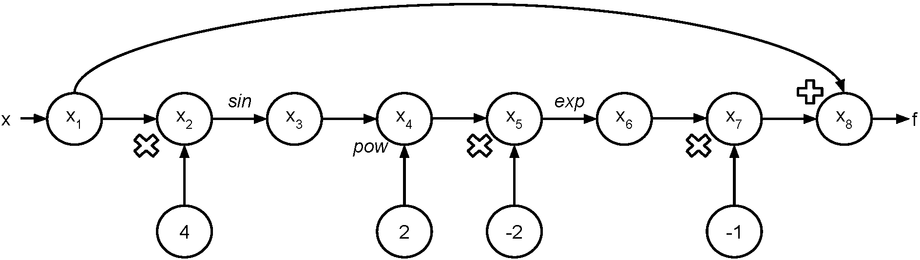
Consider again the example function $$f\left(x\right) = x - \exp\left(-2\sin^{2}\left(4x\right)\right).$$ We'd like to evalute $f$ at the point $a$.
- First, we'll generate the "evaluation trace".
- Then we'll generate the "evaluation graph". In the graph, we indicate the input value as $x$ and the output value as $f$. Note that $x$ should take on whatever value you want it to.
Let's find $f\left(\dfrac{\pi}{16}\right)$. The evaluation trace looks like:
| Trace | Elementary Operation | Numerical Value |
|---|---|---|
| $x_{1}$ | $\dfrac{\pi}{16}$ | $\dfrac{\pi}{16}$ |
| $x_{2}$ | $4x_{1}$ | $\dfrac{\pi}{4}$ |
| $x_{3}$ | $\sin\left(x_{2}\right)$ | $\dfrac{\sqrt{2}}{2}$ |
| $x_{4}$ | $x_{3}^{2}$ | $\dfrac{1}{2}$ |
| $x_{5}$ | $-2x_{4}$ | $-1$ |
| $x_{6}$ | $\exp\left(x_{5}\right)$ | $\dfrac{1}{e}$ |
| $x_{7}$ | $-x_{6}$ | $-\dfrac{1}{e}$ |
| $x_{8}$ | $x_{1} + x_{7}$ | $\dfrac{\pi}{16} - \dfrac{1}{e}$ |
Recall: $f\left(x\right) = x - \exp\left(-2\sin^{2}\left(4x\right)\right).$
Of course, the computer holds floating point values. The value of $f\left(\dfrac{\pi}{16}\right)$ is $-0.17152990032208026$. We can check this with our function.
f(np.pi / 16.0)
np.pi / 16.0 - 1.0 / np.exp(1.0)
One way to visualize what is going on is to represent the evaluation trace with a graph.
Carrying Derivatives Along
Let's compute $f^{\prime}\left(\dfrac{\pi}{16}\right)$ where $f^{\prime}\left(x\right) = \dfrac{\partial f}{\partial x}$. We'll extend the table to calculate the derivatives as we go along. Note that here the overdot $\dot{\left(\cdot\right)}$ signifies a derivative of an elemental function with respect to its argument.
| Trace | Elementary Operation | Derivative | $\left(f\left(a\right), f^{\prime}\left(a\right)\right)$ |
|---|---|---|---|
| $x_{1}$ | $\dfrac{\pi}{16}$ | $1$ | $\left(\dfrac{\pi}{16}, 1\right)$ |
| $x_{2}$ | $4x_{1}$ | $4\dot{x}_{1}$ | $\left(\dfrac{\pi}{4}, 4\right)$ |
| $x_{3}$ | $\sin\left(x_{2}\right)$ | $\cos\left(x_{2}\right)\dot{x}_{2}$ | $\left(\dfrac{\sqrt{2}}{2}, 2\sqrt{2}\right)$ |
| $x_{4}$ | $x_{3}^{2}$ | $2x_{3}\dot{x}_{3}$ | $\left(\dfrac{1}{2}, 4\right)$ |
| $x_{5}$ | $-2x_{4}$ | $-2\dot{x}_{4}$ | $\left(-1, -8\right)$ |
| $x_{6}$ | $\exp\left(x_{5}\right)$ | $\exp\left(x_{5}\right)\dot{x}_{5}$ | $\left(\dfrac{1}{e}, - \dfrac{8}{e}\right)$ |
| $x_{7}$ | $-x_{6}$ | $-\dot{x}_{6}$ | $\left(-\dfrac{1}{e}, \dfrac{8}{e}\right)$ |
| $x_{8}$ | $x_{1} + x_{7}$ | $\dot{x}_{1} + \dot{x}_{7}$ | $\left(\dfrac{\pi}{16} - \dfrac{1}{e}, 1 + \dfrac{8}{e}\right)$ |
Believe it or not, that's all there is to forward mode. Notice that at each evaluation step, we also evaluate the derivative with the chain rule. Therefore, if our function $f\left(x\right)$ is composed of elemental functions for which we know the derivatives, it is a simple task to compute the derivative.
Notes
- It is not necessary, or desirable, in practice to form the computational graph explicitly. We did so here simply to provide some intuition.
- In fact, a software implementation will perform such tasks automatically.
- Moreover, it is not necessary to store function values and derivatives at each node. Once all the children of a node have been evaluated, the parent node can discard (or overwrite) its value.
Comments
Let's reiterate what we just did. We had a function $f: \mathbb{R} \mapsto \mathbb{R}$. This function can be written as a composition of $7$ functions $$f\left(a\right) = \varphi_{7}\left(\varphi_{6}\left(\varphi_{5}\left(\varphi_{4}\left(\varphi_{3}\left(\varphi_{2}\left(\varphi_{1}\left(a\right)\right)\right)\right)\right)\right)\right).$$ The derivative becomes, by the chain rule, $$f^{\prime}\left(a\right) = \varphi_{7}^{\prime}\left(\cdot\right)\varphi_{6}^{\prime}\left(\cdot\right)\varphi_{5}^{\prime}\left(\cdot\right)\varphi_{4}^{\prime}\left(\cdot\right)\varphi_{3}^{\prime}\left(\cdot\right)\varphi_{2}^{\prime}\left(\varphi_{1}\left(a\right)\cdot\right)\varphi_{1}^{\prime}\left(a\right)$$ where the $\left(\cdot\right)$ should be apparent from the context. In the evaluation trace, we computed the elemental functions $\varphi_{i}$ as we went along with the derivatives.
Remember: $\left(\varphi\left(x\right)\right)^{\prime}$ represents the derivative of the function with respect to its input.
For example: \begin{align*} \dfrac{\mathrm{d}}{\mathrm{d}x}\varphi_{2}\left(\varphi_{1}\left(x\right)\right) = \dfrac{\mathrm{d}\varphi_{2}}{\mathrm{d}\varphi_{1}}\left(\varphi_{1}\left(x\right)\right)\dfrac{\mathrm{d}\varphi_{1}}{\mathrm{d}x}\left(x\right) = \varphi_{2}^{\prime}\left(\varphi_{1}\left(x\right)\right)\varphi_{1}^{\prime}\left(x\right) \end{align*}
Exercise
You will work with the following function for this exercise, \begin{align} f\left(x,y\right) = \exp\left(-\left(\sin\left(x\right) - \cos\left(y\right)\right)^{2}\right). \end{align}
- Draw the computational graph for the function.
- Note: This graph will have $2$ inputs.
- Create the evaluation trace for this function.
- Use the graph / trace to evaluate $f\left(\dfrac{\pi}{2}, \dfrac{\pi}{3}\right)$.
- Compute $\dfrac{\partial f}{\partial x}\left(\dfrac{\pi}{2}, \dfrac{\pi}{3}\right)$ and $\dfrac{\partial f}{\partial y}\left(\dfrac{\pi}{2}, \dfrac{\pi}{3}\right)$ using the forward mode of AD.
Hints:
- $\sin\left(\dfrac{\pi}{3}\right) = \dfrac{\sqrt{3}}{2}$, $\cos\left(\dfrac{\pi}{3}\right) = \dfrac{1}{2}$
- When calculating $\dot{x}_{1}$ with respect to $y$ we say $\dot{x}_{1} = 0$ and $\dot{x}_{2} = 1$.
- Feel free to combine steps 3 and 4.
Start of evaluation trace:
| Trace | Elementary Function | Current Value | Elementary Function Derivative | $\nabla_{x}$ Value | $\nabla_{y}$ Value |
|---|---|---|---|---|---|
| $x_{1}$ | $x_{1}$ | $\dfrac{\pi}{2}$ | $\dot{x}_{1}$ | $1$ | $0$ |
| $x_{2}$ | $x_{2}$ | $\dfrac{\pi}{3}$ | $\dot{x}_{2}$ | $0$ | $1$ |
Just Beyond the Basics
Comments on Notation
The "dot" notation is somewhat standard notation in the AD community (as much as any terminology is standard in the AD community). You should feel free to use whatever notation makes you happy in this class. Note, too, that when we start into the reverse mode, the intermediate steps are no longer denoted by a "dot". In the reverse mode, intermediate steps are denoted with an "overbar". This differing notation helps in distinguishing the two modes.
Towards the Jacobian Matrix
Time to take a step back and recap. In the very beginning of the lecture, we motivated calculation of derivatives by Newton's method for solving a system of nonlinear equations. One of the key elements in that method is the Jacobian matrix $J = \dfrac{\partial f_{i}}{\partial x_{j}}$. So far, you have learned how to manually perform the forward mode of automatic differentiation both for scalar functions of a single variable and scalar functions of multiple variables. The solution of systems of equations requires differentation of a vector-function of multiple variables.
Some Notation and the Seed Vector
Note that every time we computed the derivative using the forward mode, we "seeded" the derivative with a value.
We chose this value to be $1$.
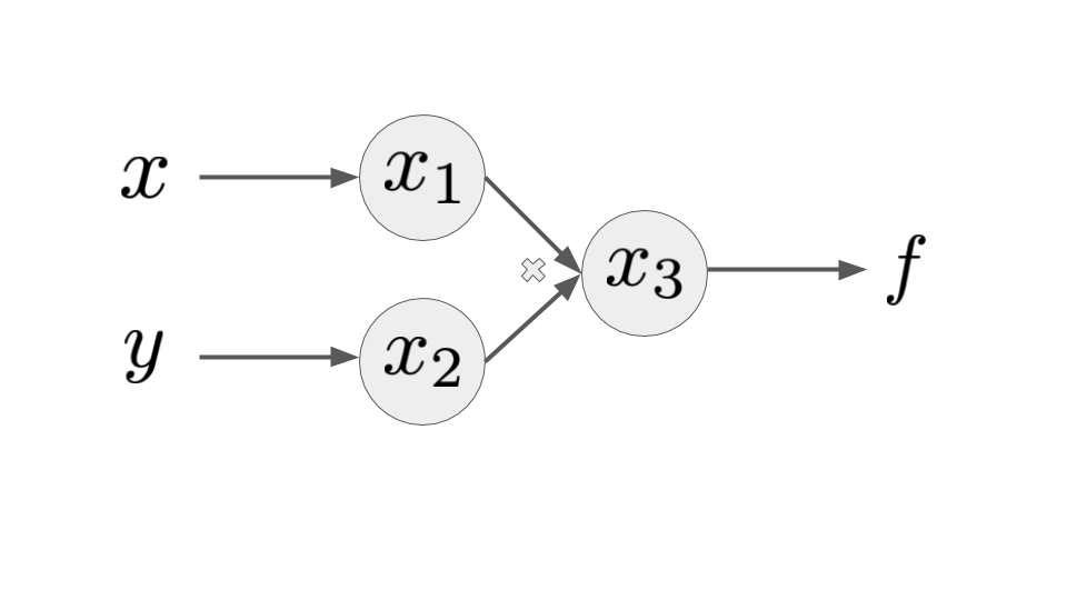
Let's look at a very simple function $f\left(x,y\right) = xy$.
Clearly $\nabla f = \begin{bmatrix} y \\ x \end{bmatrix}$ for $f\left(x,y\right) = xy$.
The evaluation trace consists of $f = x_{3} = x_{1}x_{2}$.
Let's introduce a seed vector $p$ and recall the definition of the directional derivative to be $$D_{p}x_{3} = \sum_{j=1}^{2}{\dfrac{\partial x_{3}}{\partial x_{j}}p_{j}}.$$
This tells us the derivative of $x_{3}$ ($f$) in the direction of $p$.
Expanding the sum gives \begin{align} D_{p}x_{3} &= \dfrac{\partial x_{3}}{\partial x_{1}}p_{1} + \dfrac{\partial x_{3}}{\partial x_{2}}p_{2} \\ &= x_{2}p_{1} + x_{1}p_{2}. \end{align}
Two choices for $p$:
- $p = \left(1,0\right)$ gives us $\dfrac{\partial f}{\partial x}$
- $p = \left(0,1\right)$ gives us $\dfrac{\partial f}{\partial y}$
Of course, we aren't required to choose the seed vectors to be unit vectors. However, the utility should be apparent.
Note that this could be written as $$D_{p}x_{3} = \nabla x_{3}\cdot p.$$ So, the forward mode of AD is really computing the product of the gradient of our function with the seed vector!
Towards the Jacobian
Time to take a step back and recap. In the very beginning of the lecture, we motivated calculation of derivatives by Newton's method for solving a system of nonlinear equations. One of the key elements in that method is the Jacobian matrix $J = \dfrac{\partial f_{i}}{\partial x_{j}}$. So far, you have learned how to manually perform the forward mode of automatic differentiation both for scalar functions of a single variable and scalar functions of multiple variables. The solution of systems of equations requires differentation of a vector-function of multiple variables.
Some Notation and the Seed Vector
Note that every time we computed the derivative using the forward mode, we "seeded" the derivative with a value. We chose this value to be $1$. Let's look at a very simple function $f\left(x,y\right) = xy$. Clearly $$\nabla f = \begin{bmatrix} y \\ x \end{bmatrix}.$$ The evaluation trace consists of $f = x_{3} = x_{1}x_{2}$ where $x_{1}$ and $x_{2}$ take on the values at the point we wish to evaluate the function and its derivative. Let's introduce a seed vector $p$ and define the directional derivative to be $$D_{p}x_{3} = \sum_{j=1}^{2}{\dfrac{\partial x_{3}}{\partial x_{j}}p_{j}}.$$ Expanding the sum gives \begin{align} D_{p}x_{3} &= \dfrac{\partial x_{3}}{\partial x_{1}}p_{1} + \dfrac{\partial x_{3}}{\partial x_{2}}p_{2} \\ &= x_{2}p_{1} + x_{1}p_{2}. \end{align} Notice that if we choose the seed vector to be $p = \left(1,0\right)$ we get $\dfrac{\partial f}{\partial x}$ and if we choose $p = \left(0,1\right)$ we get $\dfrac{\partial f}{\partial y}$. Of course, we aren't required to choose the seed vectors to be unit vectors. However, the utility should be apparent.
Note that this could be written as $$D_{p}x_{3} = \nabla x_{3}\cdot p.$$ So, the forward mode of AD is really computing the product of the gradient of our function with the seed vector!
What Forward AD Actually Computes
The forward mode of automatic differentiation actually computes the product $\nabla f \cdot p$. If $f$ is a vector, then the forward mode actually computes $Jp$ where $J = \dfrac{\partial f_{i}}{\partial x_{j}}, \quad i = 1,\ldots, n, \quad j = 1,\ldots,m$ is the Jacobian matrix. In many applications, we really only want the "action" of the Jacobian on a vector. That is, we just want to compute the matrix-vector product $Jp$ for some vector $p$. Of course, if we really want to form the entire Jacobian, this is readily performed by forming a set of $m$ unit seed vectors $\left\{p_{1},\ldots p_{m}\right\}$ where $p_{k}$ consists of all zeros except for a single $1$ in position $k$.
What Forward AD Actually Computes
The forward mode of automatic differentiation actually computes the product $\nabla f \cdot p$.
If $f$ is a vector, then the forward mode actually computes $Jp$ where $J = \dfrac{\partial f_{i}}{\partial x_{j}}, \quad i = 1,\ldots, n, \quad j = 1,\ldots,m$ is the Jacobian matrix.
In many applications, we really only want the "action" of the Jacobian on a vector. That is, we just want to compute the matrix-vector product $Jp$ for some vector $p$.
Of course, if we really want to form the entire Jacobian, this is readily performed by forming a set of $m$ unit seed vectors $\left\{p_{1},\ldots p_{m}\right\}$ where $p_{k}\in \mathbb{R}^{m}$ consists of all zeros except for a single $1$ in position $k$.
Exercise
That was a lot of jargon. Let's do a little example to give the basic ideas. Let \begin{align} f\left(x,y\right) = \begin{bmatrix} xy + \sin\left(x\right) \\ x + y + \sin\left(xy\right) \end{bmatrix}. \end{align}
The computational graph will have two inputs $x$ and $y$ and two outputs, this time $x_{7}$ and $x_{8}$.
In the notation below $x_{7}$ corresponds to $f_{1}$ and $x_{8}$ corresponds to $f_{2}$.
Let's start by computing the gradient of $f_{1}$. Using the directional derivative we have \begin{align} D_{p}x_{7} = \left(\cos\left(x_{1}\right) + x_{2}\right)p_{1} + x_{1}p_{2}. \end{align} Note: You should fill in the details!
- Draw the graph
- Write out the trace
- You can do this by evaluating the function at $\left(a,b\right)$, although this isn't strictly necessary for this problem.
Choosing $p = (1,0)$ gives $\dfrac{\partial f_{1}}{\partial x}$ and choosing $p = (0,1)$ gives $\dfrac{\partial f_{1}}{\partial y}$.
These form the first row of the Jacobian! The second row of the Jacobian can be computed similarly by working with $x_{8}$.
The take-home message is that we can form the full Jacobian by using $m$ seed vectors where $m$ is the number of independent variables.
This is independent of the number of functions!
Exercise
That was a lot of jargon. Let's do a little example to give the basic ideas. Let \begin{align} f\left(x,y\right) = \begin{bmatrix} xy + \sin\left(x\right) \\ x + y + \sin\left(xy\right) \end{bmatrix}. \end{align} The computational graph will have two inputs $x$ and $y$ and two outputs this time $x_{7}$ and $x_{8}$. In the notation below $x_{7}$ corresponds to $f_{1}$ and $x_{8}$ corresponds to $f_{2}$. Let's start by computing the gradient of $f_{1}$. Using the directional derivative we have \begin{align} D_{p}x_{7} = \left(\cos\left(x_{1}\right) + x_{2}\right)p_{1} + x_{1}p_{2}. \end{align} Note: You should fill in the details! Choosing $p = (1,0)$ gives $\dfrac{\partial f_{1}}{\partial x}$ and choosing $p = (0,1)$ gives $\dfrac{\partial f_{1}}{\partial y}$. These form the first row of the Jacobian! The second row of the Jacobian can be computed similarly by working with $x_{8}$.
The take-home message is that we can form the full Jacobian by using $m$ seed vectors where $m$ is the number of independent variables.
Automatic Differentiation and Dual Numbers
A dual number is an extension of the real numbers. Written out, the form looks similar to a complex number.
Review of Complex Numbers
Recall that a complex number has the form $$z = a + ib$$ where we define the number $i$ so that $i^{2} = -1$.
No real number has this property but it is a useful property for a number to have. Hence the introduction of complex numbers.
Visually, you can think of a real number as a number lying on a straight line. Then, we "extend" the real line "up". The new axis is called the imaginary axis.
Complex numbers have several properties that we can use.
- Complex conjugate: $z^{*} = a - ib$.
- Magnitude of a complex number: $\left|z\right|^{2} = zz^{*} = \left(a+ib\right)\left(a-ib\right) = a^{2} + b^{2}$.
- Polar form: $z = \left|z\right|\exp\left(i\theta\right)$ where $\displaystyle \theta = \tan^{-1}\left(\dfrac{b}{a}\right)$.
Towards Dual Numbers
A dual number has a real part and a dual part. We write $$z = a + \epsilon b$$ and refer to $b$ as the dual part.
We define the number $\epsilon$ so that $\epsilon^{2} = 0$.
This does not mean that $\epsilon$ is zero! $\epsilon$ is not a real number.
Some properties of dual numbers:
- Conjugate: $z^{*} = a - \epsilon b$.
- Magnitude: $\left|z\right|^{2} = zz^{*} = \left(a+\epsilon b\right)\left(a-\epsilon b\right) = x^{2}$.
- Polar form: $z = a\left(1 + \dfrac{b}{a}\right)$.
Example
Recall that the derivative of $y=x^{2}$ is $y^{\prime} = 2x$.
Now if we extend $x$ so that it has a real part and a dual part ($x\leftarrow a + \epsilon b$) and evaluate $y$ we have \begin{align} y &= \left(a + \epsilon b\right)^{2} \\ &= x^{2} + 2ab\epsilon + \underbrace{b^{2}\epsilon^{2}}_{=0} \\ &= a^{2} + 2ab\epsilon. \end{align}
Notice that the dual part contains the derivative of our function evaluated at $a$!!
Example
Evaluate $y = \sin\left(x\right)$ when $x\leftarrow a + \epsilon b$.
We have \begin{align} y & = \sin\left(a + \epsilon b\right) \\ & = \sin\left(a\right)\cos\left(\epsilon b\right) + \cos\left(a\right)\sin\left(\epsilon b\right). \end{align}
Expanding $\cos$ and $\sin$ in their Taylor series gives \begin{align} \sin\left(\epsilon b\right) &= \sum_{n=0}^{\infty}{\left(-1\right)^{n}\dfrac{\left(\epsilon b\right)^{2n+1}}{\left(2n+1\right)!}} = \epsilon b + \dfrac{\left(\epsilon b\right)^{3}}{3!} + \cdots = \epsilon b \\ \cos\left(\epsilon b\right) &= \sum_{n=0}^{\infty}{\left(-1\right)^{n}\dfrac{\left(\epsilon b\right)^{2n}}{\left(2n\right)!}} = 1 + \dfrac{\left(\epsilon b\right)^{2}}{2} + \cdots = 1. \end{align} Note that the definition of $\epsilon$ was used which resulted in the collapsed sum.
So we see that \begin{align} y & = \sin\left(a\right) + \cos\left(a\right) b \epsilon. \end{align} And once again the real component is the function and the dual component is the derivative.
Automatic Differentiation and Dual Numbers
A dual number is an extension of the real numbers. Written out, the form looks similar to a complex number.
Review of Complex Numbers
Recall that a complex number has the form $$z = a + ib$$ where we define the number $i$ so that $i^{2} = -1$. No real number has this property but it is a useful property for a number to have. Hence the introduction of complex numbers. Visually, you can think of a real number as a number lying on a straight line. Then, we "extend" the real line "up". The new axis is called the imaginary axis.
Complex numbers have several properties that we can use.
- Complex conjugate: $z^{*} = a - ib$.
- Magnitude of a complex number: $\left|z\right|^{2} = zz^{*} = \left(a+ib\right)\left(a-ib\right) = a^{2} + b^{2}$.
- Polar form: $z = \left|z\right|\exp\left(i\theta\right)$ where $\displaystyle \theta = \tan^{-1}\left(\dfrac{b}{a}\right)$.
Towards Dual Numbers
A dual number has a real part and a dual part. We write $$z = a + \epsilon b$$ and refer to $b$ as the dual part. We define the number $\epsilon$ so that $\epsilon^{2} = 0$. This does not mean that $\epsilon$ is zero! $\epsilon$ is not a real number.
Some properties of dual numbers:
- Conjugate: $z^{*} = a - \epsilon b$.
- Magnitude: $\left|z\right|^{2} = zz^{*} = \left(a+\epsilon b\right)\left(a-\epsilon b\right) = x^{2}$.
- Polar form: $z = a\left(1 + \dfrac{b}{a}\right)$.
Example
Recall that the derivative of $y=x^{2}$ is $y^{\prime} = 2x$.
Now if we extend $x$ so that it has a real part and a dual part ($x\leftarrow a + \epsilon a$) and evaluate $y$ we have \begin{align} y &= \left(a + \epsilon b\right)^{2} \\ &= a^{2} + 2ab\epsilon + \underbrace{b^{2}\epsilon^{2}}_{=0} \\ &= a^{2} + 2ab\epsilon. \end{align}
Notice that the dual part contains the derivative of our function!!
Example
Evaluate $y = \sin\left(x\right)$ when $x\leftarrow a + \epsilon b$.
We have \begin{align} y & = \sin\left(a + \epsilon b\right) \\ & = \sin\left(a\right)\cos\left(\epsilon b\right) + \cos\left(a\right)\sin\left(\epsilon b\right). \end{align} Expanding $\cos$ and $\sin$ in their Taylor series gives \begin{align} \sin\left(\epsilon b\right) &= \sum_{n=0}^{\infty}{\left(-1\right)^{n}\dfrac{\left(\epsilon b\right)^{2n+1}}{\left(2n+1\right)!}} = \epsilon b + \dfrac{\left(\epsilon b\right)^{3}}{3!} + \cdots = \epsilon b \\ \cos\left(\epsilon b\right) &= \sum_{n=0}^{\infty}{\left(-1\right)^{n}\dfrac{\left(\epsilon b\right)^{2n}}{\left(2n\right)!}} = 1 + \dfrac{\left(\epsilon b\right)^{2}}{2} + \cdots = 1. \end{align} Note that the definition of $\epsilon$ was used which resulted in the collapsed sum.
So we see that \begin{align} y & = \sin\left(a\right) + \cos\left(a\right) b \epsilon. \end{align} And once again the real component is the function and the dual component is the derivative.
Exercise
Using dual numbers, find the derivative of $$ y = e^{x^{2}}.$$ Show your work!