Key Word(s): ??
 Data Science 2: Advanced Topics in Data
Science
Section 3: Recurrent Neural Networks
Harvard University
Spring 2021
Instructors: Mark Glickman, Pavlos Protopapas, and Chris Tanner
Authors: Chris Gumb and Eleni Kaxiras
## RUN THIS CELL TO PROPERLY HIGHLIGHT THE EXERCISES
import requests
from IPython.core.display import HTML
styles = requests.get("https://raw.githubusercontent.com/Harvard-IACS/2019-CS109B/master/content/styles/cs109.css").text
HTML(styles)
Learning Objectives
By the end of this lab, you should understand:
- how to perform basic preprocessing on text data
- the layers used in
kerasto construct RNNs and its variants (GRU, LSTM) - how the model's task (i.e., many-to-1, many-to-many) affects architecture choices
import tensorflow as tf
from tensorflow.keras.datasets import imdb
from tensorflow.keras.models import Sequential, Model, load_model
from tensorflow.keras.layers import BatchNormalization, Bidirectional, Dense, Embedding, GRU, LSTM, SimpleRNN,\
                                    Input, TimeDistributed, Dropout, RepeatVector
from tensorflow.keras.layers import Conv1D, Conv2D, Flatten, MaxPool1D, MaxPool2D, Lambda
from tensorflow.keras.callbacks import EarlyStopping, LambdaCallback, ModelCheckpoint
from tensorflow.keras.initializers import Constant
from tensorflow.keras.preprocessing import sequence
from sklearn.model_selection import train_test_split
import tensorflow_datasets
from matplotlib import pyplot as plt
import numpy as np
import pandas as pd
import re, sys
# fix random seed for reproducibility
np.random.seed(109)
Case Study: IMDB Review Classifier
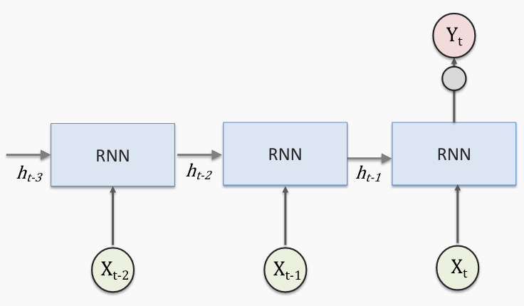
Let's frame our discussion of RNNS around the example a text classifier. Specifically, We'll build and evaluate various models that all attempt to descriminate between positive and negative reviews through the Internet Movie Database (IMDB). The dataset is again made available to us through the tensorflow datasets API.
import tensorflow_datasets
(train, test), info = tensorflow_datasets.load('imdb_reviews', split=['train', 'test'], with_info=True)
The helpful info object provides details about the dataset.
info
We see that the dataset consists of text reviews and binary good/bad labels. Here are two examples:
labels = {0: 'bad', 1: 'good'}
seen = {'bad': False, 'good': False}
for review in train:
    label = review['label'].numpy()
    if not seen[labels[label]]:
        print(f"text:\n{review['text'].numpy().decode()}\n")
        print(f"label: {labels[label]}\n")
        seen[labels[label]] = True
    if all(val == True for val in seen.values()):
        break
Great! But unfortunately, computers can read! 📖--🤖❓
Preprocessing Text Data 
Computers have no built-in knowledge of language and cannot understand text data in any rich way that humans do -- at least not without some help! The first crucial step in natural language processing is to clean and preprocess your data so that your algorithms and models can make use of it.
We'll look at a few preprocess steps:
- tokenization
- padding
- numerical encoding
Depending on your NLP task, you may want to take additional preprocessing steps which we will not cover here. These can include:
- converting all characters to lowercase
- treating each punctuation mark as a token (e.g., , . ! ? are each separate tokens)
- removing punctuation altogether
- separating each sentence with a unique symbol (e.g.,
and) - removing words that are incredibly common (e.g., function words, (in)definite articles). These are referred to as 'stopwords').
- Lemmatizing (replacing words with their 'dictionary entry form')
- Stemming (removing grammatical morphemes)
Useful NLP Python libraries such as NLTK and spaCy provide built in methods for many of these preprocessing steps.
Tokens are the atomic units of meaning which our model will be working with. What should these units be? These could be characters, words, or even sentences. For our movie review classifier we will be working at the word level.
For this example we will process just a subset of the original dataset.
SAMPLE_SIZE = 10
subset = list(train.take(SAMPLE_SIZE))
subset[0]
The TFDS format allows for the construction of efficient preprocessing pipelines. But for our own
preprocessing example we will be primarily working with Python list objects. This gives
us a chance to practice the Python list comprehension which is a powerful tool to
have at your disposal. It will serve you well when processing arbitrary text which may not already
be in a nice TFDS format (such as in the HW 😉).
We'll convert our data subset into X and y lists.
X = [x['text'].numpy().decode() for x in subset]
y = [x['label'].numpy() for x in subset]
print(f'X has {len(X)} reviews')
print(f'y has {len(y)} labels')
N_CHARS = 20
print(f'First {N_CHARS} characters of all reviews:\n{[x[:20]+"..." for x in X]}\n')
print(f'All labels:\n{y}')
Each observation in X is a review. A review is a str object which we can
think of as a sequence of characters. This is indeed how Python treats strings as made clear by how
we are printing 'slices' of each review in the code cell above.
We'll see a bit later that you can in fact sucessfully train a neural network on text data at the character level.
But for the moment we will work at the word level, treating the word level. This means our observations should be organized as sequences of words rather than sequences of characters.
# list comprehensions again to the rescue!
X = [x.split() for x in X]
# The same thing can be accomplished with:
# list(map(str.split, X))
# but that is much harder to parse! O_o
Now let's look at the first 10 tokens in the first 2 reviews.
X[0][:10], X[1][:10]
Let's take a look at the lengths of the reviews in our subset.
[len(x) for x in X]
If we were training our RNN one sentence at a time, it would be okay to have sentences of varying lengths. However, as with any neural network, it can be sometimes be advantageous to train inputs in batches. When doing so with RNNs, our input tensors need to be of the same length/dimensions.
Here are two examples of tokenized reviews padded to have a length of 5.
['I', 'loved', 'it', '', '']
['It', 'stinks', '', '', '']
Now let's pad our own examples. Note that 'padding' in this context also means truncating sequences that are longer than our specified max length.
MAX_LEN = 500
PAD = ''
# truncate
X = [x[:MAX_LEN] for x in X]
# pad
for x in X:
    while len(x) < MAX_LEN:
        x.append(PAD)
[len(x) for x in X]
Now all reviews are of a uniform length!
If each review in our dataset is an observation, then the features of each observation are the tokens, in this case, words. But these words are still strings. Our machine learning methods require us to be able to multiple our features by weights. If we want to use these words as inputs for a neural network we'll have to convert them into some numerical representation.
One solution is to create a one-to-one mapping between unique words and integers.
If the five sentences below were our entire corpus, our conversion would look this:
- i have books - [1, 4, 2]
- interesting books are useful [11,2,9,8]
- i have computers [1,4,3]
- computers are interesting and useful [3,5,11,10,8]
- books and computers are both valuable. [2,10,3,9,13,12]
- bye bye [7,7]
I-1, books-2, computers-3, have-4, are-5, computers-6,bye-7, useful-8, are-9, and-10,interesting-11, valuable-12, both-13
To accomplish this we'll first need to know what all the unique words are in our dataset.
all_tokens = [word for review in X for word in review]
# sanity check
len(all_tokens), sum([len(x) for x in X])
Casting our list of words into a set is a great way to get all the unique
words in the data.
vocab = sorted(set(all_tokens))
print('Unique Words:', len(vocab))
Now we need to create a mapping from words to integers. For this will a dictionary comprehension.
word2idx = {word: idx for idx, word in enumerate(vocab)}
word2idx
We repeat the process, this time mapping integers to words.
idx2word = {idx: word for idx, word in enumerate(vocab)}
idx2word
Now, perform the mapping to encode the observations in our subset. Note the use of nested list comprehensions!
X_proc = [[word2idx[word] for word in review] for review in X]
X_proc[0][:10], X_proc[1][:10]
X_proc is a list of lists but if we are going to feed it into a keras model
we should convert both it and y into numpy arrays.
X_proc = np.hstack(X_proc).reshape(-1, MAX_LEN)
y = np.array(y)
X_proc, y
Now, just to prove that we've successfully processed the data, we perform a test train split and feed it into a FNN.
X_train, X_test, y_train, y_test = train_test_split(X_proc, y, test_size=0.2, stratify=y)
model = Sequential()

model.add(Dense(8, activation='relu',input_dim=MAX_LEN))
model.add(Dense(1, activation='sigmoid'))
model.compile(loss='binary_crossentropy', optimizer='adam', metrics=['accuracy'])
print(model.summary())

model.fit(X_train, y_train, validation_data=(X_test, y_test), epochs=5, batch_size=2, verbose=2)

scores = model.evaluate(X_test, y_test, verbose=0)
print("Accuracy: %.2f%%" % (scores[1]*100))
It worked! But our subset was very small so we shouldn't get excited about the results above.
The IMDB dataset is very popular so keras also includes an alternative method for
loading the data. This method can save us a lot of time for many reasons:
- Cleaned text with less meaningless punctuation
- Pre-tokenized and numerically encoded
- Allows us to specify maximum vocabulary size
from tensorflow.keras.datasets import imdb
import warnings
warnings.filterwarnings('ignore')
# We want to have a finite vocabulary to make sure that our word matrices are not arbitrarily small
MAX_VOCAB = 10000
INDEX_FROM = 3   # word index offset
(X_train, y_train), (X_test, y_test) = imdb.load_data(num_words=MAX_VOCAB, index_from=INDEX_FROM)
get_word_index will load a json object we can store in a dictionary. This gives us the
word-to-integer mapping.
word2idx = imdb.get_word_index(path='imdb_word_index.json')
word2idx = {k:(v + INDEX_FROM) for k,v in word2idx.items()}
word2idx["" ] = 0
word2idx["" ] = 1
word2idx["" ] = 2
word2idx["" ] = 3
word2idx
idx2word = {v: k for k,v in word2idx.items()}
idx2word
We can see that the text data is already preprocessed for us.
print('Number of reviews', len(X_train))
print('Length of first and fifth review before padding', len(X_train[0]) ,len(X_train[4]))
print('First review', X_train[0])
print('First label', y_train[0])
Here's an example review using the index-to-word mapping we created from the loaded JSON file to view the a review in its original form.
def show_review(x):
    review = ' '.join([idx2word[idx] for idx in x])
    print(review)

show_review(X_train[0])
The only thing what isn't done for us is the padding. Looking at the distribution of lengths will help us determine what a reasonable length to pad to will be.
plt.hist([len(x) for x in X_train])
plt.title('review lengths');
We saw one way of doing this earlier, but Keras actually has a built in pad_sequences
helper function. This handles both padding and truncating. By default padding is added to the beginning
of a sequence.
from tensorflow.keras.preprocessing.sequence import pad_sequences
MAX_LEN = 500
X_train = pad_sequences(X_train, maxlen=MAX_LEN)
X_test = pad_sequences(X_test, maxlen=MAX_LEN)
print('Length of first and fifth review after padding', len(X_train[0]) ,len(X_train[4]))
Let us build a single-layer feed-forward net with a hidden layer of 250 nodes. Each input would be a 500-dim vector of tokens since we padded all our sequences to size 500.
model = Sequential(name='Naive_FFNN')
model.add(Dense(250, activation='relu',input_dim=MAX_LEN))
model.add(Dense(1, activation='sigmoid'))
model.compile(loss='binary_crossentropy', optimizer='adam', metrics=['accuracy'])
print(model.summary())

model.fit(X_train, y_train, validation_data=(X_test, y_test), epochs=10, batch_size=128, verbose=2)

scores = model.evaluate(X_test, y_test, verbose=0)
print("Accuracy: %.2f%%" % (scores[1]*100))
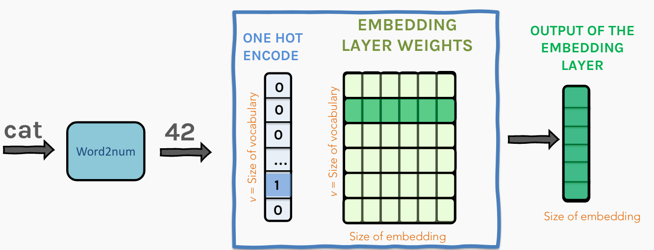
One can view the embedding process as a linear projection from one vector space to another. For NLP, we usually use embeddings to project the sparse one-hot encodings of words on to a lower-dimensional continuous space so that the input surface is 'dense' and possibly smooth. Thus, one can view this embedding layer process as just a transformation from $\mathbb{R}^{inp}$ to $\mathbb{R}^{emb}$
This not only reduces dimensionality but also allows semantic similarities between tokens to be captured by 'similiarities' between the embedding vectors. This was not possible with one-hot encoding as all vectors there were orthogonal to one another.
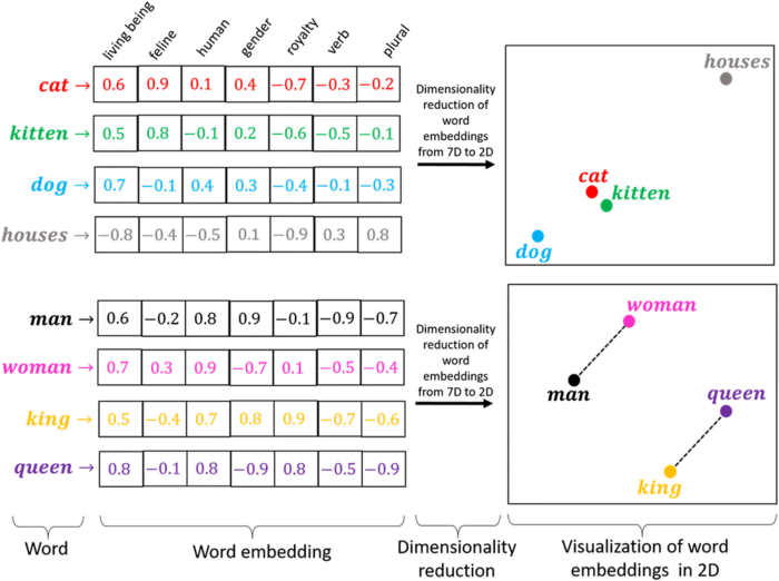
It is also possible to load pretrained embeddings that were learned from giant corpora. This would be an instance of transfer learning.
If you are interested in learning more, start with the astromonically impactful papers of word2vec and GloVe.
In Keras we use the Embedding
layer:
tf.keras.layers.Embedding(
    input_dim, output_dim, embeddings_initializer='uniform',
    embeddings_regularizer=None, activity_regularizer=None,
    embeddings_constraint=None, mask_zero=False, input_length=None, **kwargs
)
We'll need to specify the input_dim and output_dim. If working with
sequences, as we are, you'll also need to set the input_length.
EMBED_DIM = 100

model = Sequential(name='FFNN_EMBED')
model.add(Embedding(MAX_VOCAB, EMBED_DIM, input_length=MAX_LEN))
model.add(Flatten())
model.add(Dense(250, activation='relu'))
model.add(Dense(1, activation='sigmoid'))
model.compile(loss='binary_crossentropy', optimizer='adam', metrics=['accuracy'])
print(model.summary())

model.fit(X_train, y_train, validation_data=(X_test, y_test), epochs=2, batch_size=128, verbose=2)

scores = model.evaluate(X_test, y_test, verbose=0)
print("Accuracy: %.2f%%" % (scores[1]*100))
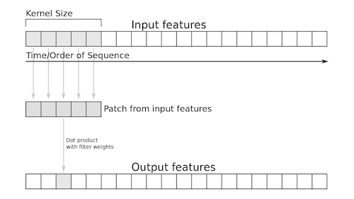
Text can be thought of as 1-dimensional sequence (a single, long vector) and we can apply 1D
Convolutions over a set of word embeddings.
More information on convolutions on text data can be found on this blog. If you want to learn more, read this published and well-cited paper from Eleni's friend, Byron Wallace.
model = Sequential(name='1D_CNN')
model.add(Embedding(MAX_VOCAB, EMBED_DIM, input_length=MAX_LEN))
model.add(Conv1D(filters=200, kernel_size=3, padding='same', activation='relu'))
model.add(MaxPool1D(pool_size=2))
model.add(Flatten())
model.add(Dense(250, activation='relu'))
model.add(Dense(1, activation='sigmoid'))
model.compile(loss='binary_crossentropy', optimizer='adam', metrics=['accuracy'])
print(model.summary())

model.fit(X_train, y_train, epochs=2, batch_size=128)

scores = model.evaluate(X_test, y_test, verbose=0)
print("Accuracy: %.2f%%" % (scores[1]*100))
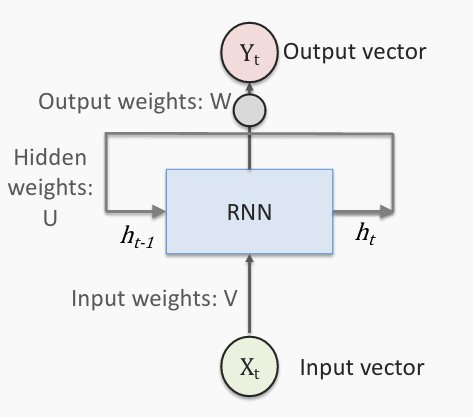
At a high-level, an RNN is similar to a feed-forward neural network (FFNN) in that there is an input layer, a hidden layer, and an output layer. The input layer is fully connected to the hidden layer, and the hidden layer is fully connected to the output layer. However, the crux of what makes it a recurrent neural network is that the hidden layer for a given time t is not only based on the input layer at time t but also the hidden layer from time t-1.
Here's a popular blog post on The Unreasonable Effectiveness of Recurrent Neural Networks.
In Keras, the vanilla RNN unit is implemented theSimpleRNN layer:
tf.keras.layers.SimpleRNN(
    units, activation='tanh', use_bias=True,
    kernel_initializer='glorot_uniform',
    recurrent_initializer='orthogonal',
    bias_initializer='zeros', kernel_regularizer=None,
    recurrent_regularizer=None, bias_regularizer=None, activity_regularizer=None,
    kernel_constraint=None, recurrent_constraint=None, bias_constraint=None,
    dropout=0.0, recurrent_dropout=0.0, return_sequences=False, return_state=False,
    go_backwards=False, stateful=False, unroll=False, **kwargs
)
As you can see, recurrent layers in Keras take many arguments. We only need to be concerned with
units, which specifies the size of the hidden state, and return_sequences,
which will be discussed shortly. For the moment is it fine to leave this set to the default of
False.
Due to the limitations of the vanilla RNN unit (more on that next) it tends not to be used much in practice. For this reason it seems that the Keras developers neglected to implement GPU acceleration for this layer! Notice how much slower the trainig is even for a network with far fewer parameters.
model = Sequential(name='SimpleRNN')
model.add(Embedding(MAX_VOCAB, EMBED_DIM, input_length=MAX_LEN))
model.add(SimpleRNN(100))
model.add(Dense(1, activation='sigmoid'))
model.compile(loss='binary_crossentropy', optimizer='adam', metrics=['accuracy'])
print(model.summary())

model.fit(X_train, y_train, epochs=3, batch_size=128)

scores = model.evaluate(X_test, y_test, verbose=0)
print("Accuracy: %.2f%%" % (scores[1]*100))

We need to backpropogate through every time step to calculate the gradients used for our weight updates.
This requires the use of the chain rule which amounts to repeated multiplications.
This can cause two types of problems. First, this product can quickly 'explode,' becoming large, causing destructive updates to the model and numerical overflow. One hack to solve this problem is to clip the gradient at some threshold.
Alternatively, the gradient can 'vanish,' getting smaller and smaller as the gradient moves backwards in time. Gradient clipping will not help us here. If we can't propogate gradients suffuciently far back in time then our network will be unable to learn long temporal dependencies. This problem motivates the architecture of the GRU and LSTM units as substitutes for the 'vanilla' RNN.
For a more detailed look at the vanishing/exploding gradient problem, please see Marios's excellent Advanced Section.
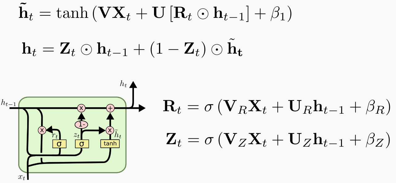
$X_{t}$: input
$U$, $V$, and $\beta$: parameter matrices and vector
$\tilde{h_t}$: candidate activation vector
$h_{t}$: output vector
$R_t$: reset gate
$Z_t$: update gate
The gates of the GRU allow for the gradients to flow more freely to previous time steps, helping to mitigate the vanishing gradient problem.
In Keras, the GRU layer
is used in exactly the same way as the SimpleRNN layer.
tf.keras.layers.GRU(
    units, activation='tanh', recurrent_activation='sigmoid',
    use_bias=True, kernel_initializer='glorot_uniform',
    recurrent_initializer='orthogonal',
    bias_initializer='zeros', kernel_regularizer=None,
    recurrent_regularizer=None, bias_regularizer=None, activity_regularizer=None,
    kernel_constraint=None, recurrent_constraint=None, bias_constraint=None,
    dropout=0.0, recurrent_dropout=0.0, return_sequences=False, return_state=False,
    go_backwards=False, stateful=False, unroll=False, time_major=False,
    reset_after=True, **kwargs
)
Here we just swap it in to the previous architecture. Note how much faster it trains with GPU excelleration than the simple RNN!
model = Sequential(name='GRU')
model.add(Embedding(MAX_VOCAB, EMBED_DIM, input_length=MAX_LEN))
model.add(GRU(100))
model.add(Dense(1, activation='sigmoid'))
model.compile(loss='binary_crossentropy', optimizer='adam', metrics=['accuracy'])
print(model.summary())

model.fit(X_train, y_train, epochs=3, batch_size=64)

scores = model.evaluate(X_test, y_test, verbose=0)
print("Accuracy: %.2f%%" % (scores[1]*100))
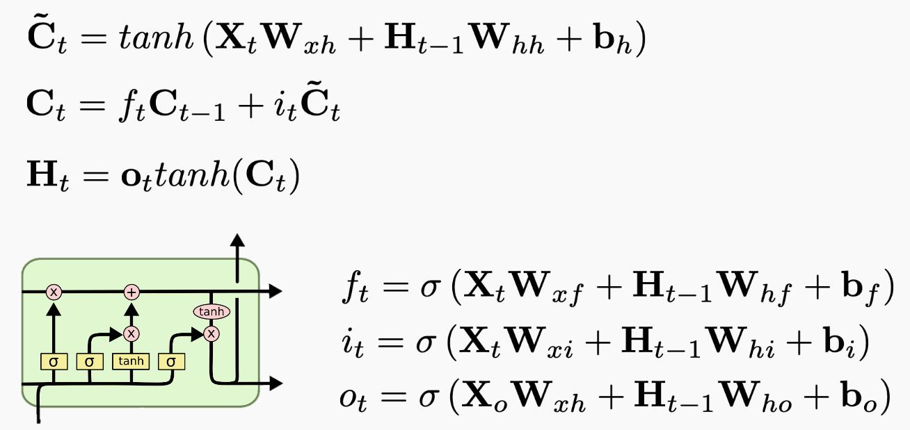
The LSTM lacks the GRU's 'short cut' connection (see GRU's $h_t$ above).
The LSTM also has a distinct 'cell state' in addition to the hidden state.
Futher reading:
- Understanding LSTM Networks
- LSTM: A Search Space Odyssey
- An Empirical Exploration of Recurrent Network Architectures
Again, Kera's LSTM
works like all the other recurrent layers.
tf.keras.layers.LSTM(
    units, activation='tanh', recurrent_activation='sigmoid',
    use_bias=True, kernel_initializer='glorot_uniform',
    recurrent_initializer='orthogonal',
    bias_initializer='zeros', unit_forget_bias=True,
    kernel_regularizer=None, recurrent_regularizer=None, bias_regularizer=None,
    activity_regularizer=None, kernel_constraint=None, recurrent_constraint=None,
    bias_constraint=None, dropout=0.0, recurrent_dropout=0.0,
    return_sequences=False, return_state=False, go_backwards=False, stateful=False,
    time_major=False, unroll=False, **kwargs
)model = Sequential(name='LSTM')
model.add(Embedding(MAX_VOCAB, EMBED_DIM, input_length=MAX_LEN))
model.add(LSTM(100))
model.add(Dense(1, activation='sigmoid'))
model.compile(loss='binary_crossentropy', optimizer='adam', metrics=['accuracy'])
print(model.summary())
model.fit(X_train, y_train, epochs=3, batch_size=64)
scores = model.evaluate(X_test, y_test, verbose=0)
print("Accuracy: %.2f%%" % (scores[1]*100))
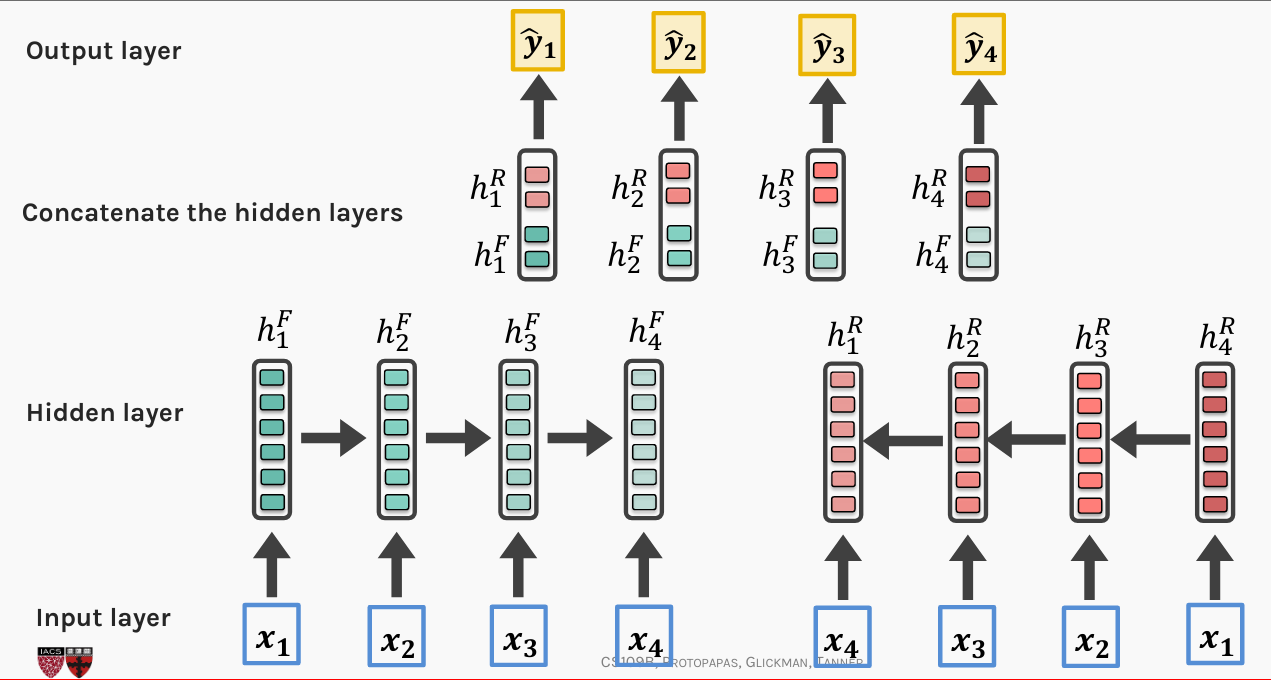
We may want our model to learn dependencies in either direction. A BiDirectional RNN
consists of two separate recurrent units. One processing the sequence from left to right, the other
processes that same sequence but in reverse, from right to left. The output of the two units are
then merged together (typically concatenated) and feed to the next layer of the network.
Creating a Bidirection RNN in Keras is quite simple. We just 'wrap' a recurrent layer in the Bidirectional
layer. The default behavior is to concatenate the output from each direction.
tf.keras.layers.Bidirectional(
    layer, merge_mode='concat', weights=None, backward_layer=None,
    **kwargs
)
Example:
model = Sequential()
...
model.add(Bidirectional(SimpleRNN(n_nodes))
...
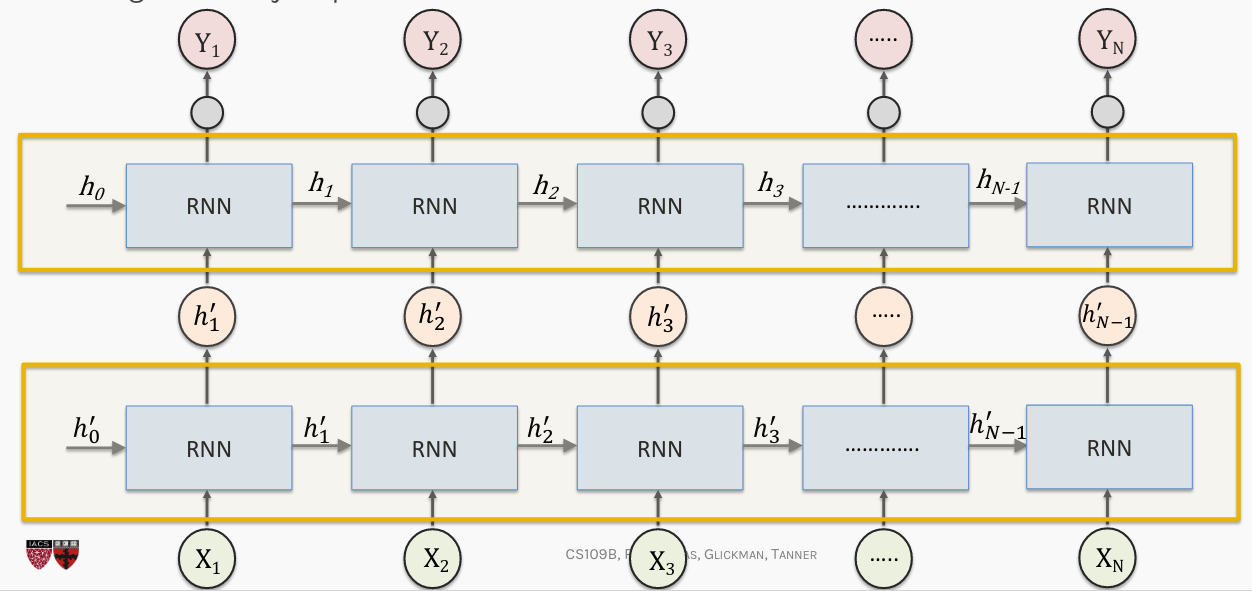
We may want to stack RNN layers one after another. But there is a problem. A recurrent layer expects to be given a sequence as input, and yet we can see that the recurrent layer in each of our models above outputs a single vector. This is because the default behavior of Keras's recurrent layers is to suppress the output until the final time step. If we want to have two recurrent units in a row then the first will have to given an output after each time step, thus providing a sequence to the 2nd recurrent layer.
We can have our recurrent layers output at each time step setting return_sequences=True.
Example:
model = Sequential()
...
model.add(LSTM(100, return_sequences=True))
model.add(LSTM(100)
...
TimeDistributed
is a 'wrapper' that applies a layer to all time steps of an input sequence.
tf.keras.layers.TimeDistributed(
    layer, **kwargs
)
We use TimeDistributed when we want to input a sequence into a layer that doesn't
normally expect a time dimension, such as Dense.
model = Sequential()
model.add(TimeDistributed(Dense(8), input_shape=(3, 5)))
input_array = np.random.randint(10, size=(1,3,5))
print("Shape of input : ", input_array.shape)

model.compile('rmsprop', 'mse')
output_array = model.predict(input_array)
print("Shape of output : ", output_array.shape)
RepeatVector
repeats the vector a specified number of times. Dimension changes from
(batch_size, number_of_elements)
to
(batch_size, number_of_repetitions, number_of_elements)
This effectively generates a sequence from a single input.
model = Sequential()
model.add(Dense(2, input_dim=1))
model.add(RepeatVector(3))
model.summary()
CNNs are good at learning spatial features, and sentences can be thought of as 1-D spatial vectors (dimensionality is determined by the number of words in the sentence). We can then take the features learned by the CNN (after a maxpooling layer) and feed them into an RNN! We expect the CNN to be able to pick out invariant features across the 1-D spatial structure (i.e., sentence) that characterize good and bad sentiment. This learned spatial features may then be learned as sequences by a reccurent layer. The classification step is then performed by a final dense layer.
Let's put together everything we've learned so far.
Create a network with:
- word embeddings in a 100-dimensional space
- conv layer with 32 filters, kernels of width 3, 'same' padding, and ReLU activate
- max pooling of size 2
- 2 bidirectional GRU layers, each with 50 units per direction
- dense output layer for binary classification
model = Sequential(name='CNN_GRU')
# your code here
model.add(Embedding(MAX_VOCAB, 100, input_length=MAX_LEN))
model.add(Conv1D(filters=32, kernel_size=3, padding='same', activation='relu'))
model.add(MaxPool1D(pool_size=2))
model.add(Bidirectional(GRU(50, return_sequences=True)))
model.add(Bidirectional(GRU(50)))
model.add(Dense(1, activation='sigmoid'))
model.compile(loss='binary_crossentropy', optimizer='adam', metrics=['accuracy'])
print(model.summary())

model.fit(X_train, y_train, epochs=3, batch_size=64)

scores = model.evaluate(X_test, y_test, verbose=0)
print("Accuracy: %.2f%%" % (scores[1]*100))
What is the worst movie review in the test set according to your model? 🍅
preds = model.predict_proba(X_test)
worst_review = X_test[preds.argmin()]
show_review(worst_review)