Key Word(s): autoencoders, AE, variational autoencoders, VAE, GANs, generative adversarial networks
 CS109B Data Science 2: Advanced Topics in Data Science
Lab 10: Variational Autoencoders and GANs
Harvard University
Fall 2020
Instructors: Mark Glickman, Pavlos Protopapas, and Chris Tanner
Lab Instructors: Chris Tanner and Eleni Angelaki Kaxiras
Content: Srivatsan Srinivasan, Pavlos Protopapas, Chris Tanner
# RUN THIS CELL TO PROPERLY HIGHLIGHT THE EXERCISES
import requests
from IPython.core.display import HTML
styles = requests.get("https://raw.githubusercontent.com/Harvard-IACS/2019-CS109B/master/content/styles/cs109.css").text
HTML(styles)
# system libraries
import sys
import warnings
import os
import glob
warnings.filterwarnings("ignore")

# image libraries
import cv2 # requires installing opencv (e.g., pip install opencv-python)
from imgaug import augmenters # requires installing imgaug (e.g., pip install imgaug)

# math/numerical libraries
import matplotlib.pyplot as plt
import numpy as np
import pandas as pd
import scipy
from scipy.stats import norm
from sklearn.model_selection import train_test_split

import tensorflow as tf

# deep learning libraries
from keras.models import Model, Sequential
from keras.optimizers import Adam, RMSprop

from keras.layers import *
from keras import backend as K
# from keras.callbacks import EarlyStopping
# from keras.utils import to_categorical
# from keras.metrics import *
# from keras.preprocessing import image, sequence
#

print(tf.__version__)
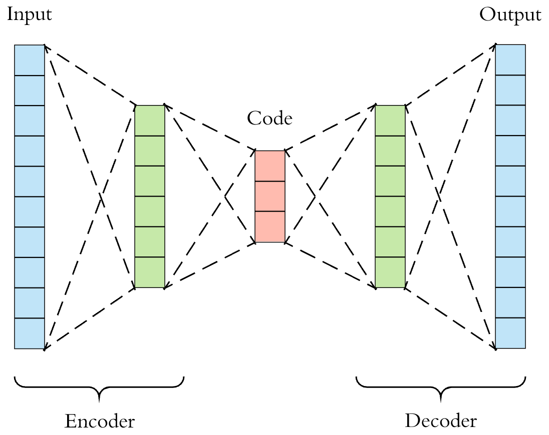
Part 1: Recap of Autoencoders (AEs)
As a reminder, this is the typical architecture of a 'vanilla/standard/traditional' autoencoder.
Data: obtainment and pre-processing
We will be using Fashion-MNIST, the same dataset that we used in Lab 7 when we studied traditional autoencoders. Again, we can conveniently access the dataset since it is included with Keras:
# get the data from keras - how convenient!
fashion_mnist = tf.keras.datasets.fashion_mnist

# load the data and split it into training and testing sets
(X_train, y_train),(X_test, y_test) = fashion_mnist.load_data()

# normalize the data by dividing with pixel intensity
# (each pixel is 8 bits so its value ranges from 0 to 255)
X_train, X_test = X_train / 255.0, X_test / 255.0

print(f'X_train shape: {X_train.shape}, X_test shape: {X_test.shape}')
print(f'y_train shape: {y_train.shape}, and y_test shape: {y_test.shape}')

# classes are named 0-9 so define names for plotting clarity
class_names = ['T-shirt/top', 'Trouser', 'Pullover', 'Dress', 'Coat',
               'Sandal', 'Shirt', 'Sneaker', 'Bag', 'Ankle boot']

# display the first 25 garments from the training set
plt.figure(figsize=(10,10))
for i in range(25):
    plt.subplot(5,5,i+1)
    plt.xticks([])
    plt.yticks([])
    plt.grid(False)
    plt.imshow(X_train[i], cmap=plt.cm.binary)
    plt.xlabel(class_names[y_train[i]])
plt.show()

Add Noise to Images
In attempt to make the autoencoder more robust and not just memorize the inputs, let's add noise to the inputs but calculate its loss based on how similar its outputs are to the original (non-denoised) images.
Check out imgaug docs for more info and other ways to add noise.
# NNs want the inputs to be 3D
n_samples, h, w = X_train.shape

X_train = X_train.reshape(-1, h, w, 1)
X_test = X_test.reshape(-1, h, w, 1)
# Lets add sample noise - Salt and Pepper
noise = augmenters.SaltAndPepper(0.1)
seq_object = augmenters.Sequential([noise])

X_train_n = seq_object.augment_images(X_train * 255) / 255
X_test_n = seq_object.augment_images(X_test * 255) / 255

f, ax = plt.subplots(1,5)
f.set_size_inches(80, 40)
for i in range(5,10):
    ax[i-5].imshow(X_train_n[i, :, :, 0].reshape(28, 28), cmap=plt.cm.binary)
    ax[i-5].set_xlabel('Clean '+class_names[y_train[i]])

Create the Autoencoder
# input layer
input_layer = tf.keras.layers.Input(shape=(28, 28, 1))

# encoding architecture
encoded_layer1 = tf.keras.layers.Conv2D(64,(3, 3), activation='relu', padding='same')(input_layer)
encoded_layer1 = tf.keras.layers.MaxPool2D((2, 2), padding='same')(encoded_layer1)
encoded_layer2 = tf.keras.layers.Conv2D(32,(3, 3), activation='relu', padding='same')(encoded_layer1)
encoded_layer2 = tf.keras.layers.MaxPool2D((2, 2), padding='same')(encoded_layer2)
encoded_layer3 = tf.keras.layers.Conv2D(16,(3, 3), activation='relu', padding='same')(encoded_layer2)
latent_view = tf.keras.layers.MaxPool2D((2, 2), padding='same')(encoded_layer3)

# decoding architecture
decoded_layer1 = tf.keras.layers.Conv2D(16, (3, 3), activation='relu', padding='same')(latent_view)
decoded_layer1 = tf.keras.layers.UpSampling2D((2, 2))(decoded_layer1)
decoded_layer2 = tf.keras.layers.Conv2D(32, (3, 3), activation='relu', padding='same')(decoded_layer1)
decoded_layer2 = tf.keras.layers.UpSampling2D((2, 2))(decoded_layer2)
decoded_layer3 = tf.keras.layers.Conv2D(64, (3, 3), activation='relu')(decoded_layer2)
decoded_layer3 = tf.keras.layers.UpSampling2D((2, 2))(decoded_layer3)
output_layer = tf.keras.layers.Conv2D(1,(3, 3), padding='same')(decoded_layer3)

# compile the model
model = tf.keras.Model(input_layer, output_layer)
model.compile(optimizer='adam', loss='mse')
model.summary()
Train AE
early_stopping = tf.keras.callbacks.EarlyStopping(monitor='val_loss', min_delta=0, patience=10, verbose=5, mode='auto')

# epochs=20 for better results
history = model.fit(X_train_n, X_train, epochs=5, batch_size=2048, validation_data=(X_test_n, X_test), callbacks=[early_stopping])
n = np.random.randint(0,len(X_test)-5) # pick a random starting index within our test set
Visualize Samples reconstructed by AE
Denoised Images:
f, ax = plt.subplots(1,5)
f.set_size_inches(80, 40)
for i,a in enumerate(range(n,n+5)):
    ax[i].imshow(X_test_n[a, :, :, 0].reshape(28, 28), cmap='gray')

Actual Targets (i.e., Original inputs):
f, ax = plt.subplots(1,5)
f.set_size_inches(80, 40)
for i,a in enumerate(range(n,n+5)): # display the 5 images starting at our random index
    ax[i].imshow(X_test[a, :, :, 0].reshape(28, 28), cmap='gray')

Predicted Images:
preds = model.predict(X_test_n[n:n+5])
f, ax = plt.subplots(1,5)
f.set_size_inches(80, 40)
for i,a in enumerate(range(n,n+5)):
    ax[i].imshow(preds[i].reshape(28, 28), cmap='gray')
plt.show()

Part 2: Variational Autoencoders (VAEs)
VAE architecture

Reset data
# get the data from keras - how convenient!
fashion_mnist = tf.keras.datasets.fashion_mnist

# load the data and split it into training and testing sets
(X_train, y_train),(X_test, y_test) = fashion_mnist.load_data()

# normalize the data by dividing with pixel intensity
# (each pixel is 8 bits so its value ranges from 0 to 255)
X_train, X_test = X_train / 255.0, X_test / 255.0

print(f'X_train shape: {X_train.shape}, X_test shape: {X_test.shape}')
print(f'y_train shape: {y_train.shape}, and y_test shape: {y_test.shape}')
#train_x = train_x.reshape(-1, 28, 28, 1)
#val_x = val_x.reshape(-1, 28, 28, 1)
Setup Encoder Neural Network
Try different number of hidden layers, nodes?
batch_size = 16
latent_dim = 2  # Number of latent dimension parameters

input_img = tf.keras.layers.Input(shape=(784,), name="input")
x = tf.keras.layers.Dense(512, activation='relu', name="intermediate_encoder")(input_img)
x = tf.keras.layers.Dense(2, activation='relu', name="latent_encoder")(x)

z_mu = tf.keras.layers.Dense(latent_dim)(x)
z_log_sigma = tf.keras.layers.Dense(latent_dim)(x)
#import keras.backend as K
# sampling function
def sampling(args):
    z_mu, z_log_sigma = args
    epsilon = tf.keras.backend.random_normal(shape=(tf.keras.backend.shape(z_mu)[0], latent_dim))
    z = z_mu + tf.keras.backend.exp(z_log_sigma) * epsilon
    return z

# sample vector from the latent distribution
z = tf.keras.layers.Lambda(sampling)([z_mu, z_log_sigma])
# decoder takes the latent distribution sample as input
decoder_input = tf.keras.layers.Input((2,), name="input_decoder")

x = tf.keras.layers.Dense(512, activation='relu', name="intermediate_decoder", input_shape=(2,))(decoder_input)

# Expand to 784 total pixels
x = tf.keras.layers.Dense(784, activation='sigmoid', name="original_decoder")(x)

# decoder model statement
decoder = tf.keras.Model(decoder_input, x)

# apply the decoder to the sample from the latent distribution
z_decoded = decoder(z)
decoder.summary()
# construct a custom layer to calculate the loss
class CustomVariationalLayer(tf.keras.layers.Layer):

    def vae_loss(self, x, z_decoded):
        x = tf.keras.backend.flatten(x)
        z_decoded = tf.keras.backend.flatten(z_decoded)
        # Reconstruction loss
        xent_loss = tf.keras.losses.binary_crossentropy(x, z_decoded)
        return xent_loss

    # adds the custom loss to the class
    def call(self, inputs):
        x = inputs[0]
        z_decoded = inputs[1]
        loss = self.vae_loss(x, z_decoded)
        self.add_loss(loss, inputs=inputs)
        return x

# apply the custom loss to the input images and the decoded latent distribution sample
y = CustomVariationalLayer()([input_img, z_decoded])
z_decoded
# VAE model statement
vae = tf.keras.Model(input_img, y)
vae.compile(optimizer='rmsprop', loss=None)
vae.summary()
X_train.shape
train_x = X_train.reshape(-1,784) # train_x.reshape(-1, 784)
val_x = X_test.reshape(-1,784) #val_x.reshape(-1, 784)
vae.fit(x=train_x, y=None,
        shuffle=True,
        epochs=4,
        batch_size=batch_size,
        validation_data=(val_x, None))
# Display a 2D manifold of the samples
n = 20  # figure with 20x20 samples
digit_size = 28
figure = np.zeros((digit_size * n, digit_size * n))

# Construct grid of latent variable values - can change values here to generate different things
grid_x = norm.ppf(np.linspace(0.05, 0.95, n))
grid_y = norm.ppf(np.linspace(0.05, 0.95, n))

# decode for each square in the grid
for i, yi in enumerate(grid_x):
    for j, xi in enumerate(grid_y):
        z_sample = np.array([[xi, yi]])
        z_sample = np.tile(z_sample, batch_size).reshape(batch_size, 2)

        x_decoded = decoder.predict(z_sample, batch_size=batch_size)

        digit = x_decoded[0].reshape(digit_size, digit_size)

        figure[i * digit_size: (i + 1) * digit_size,
               j * digit_size: (j + 1) * digit_size] = digit

plt.figure(figsize=(20, 20))
plt.imshow(figure, cmap='gray')
plt.show()

# Translate into the latent space
encoder = tf.keras.Model(input_img, z_mu) # works on older version of TF and Keras
x_valid_noTest_encoded = encoder.predict(train_x, batch_size=batch_size)
plt.figure(figsize=(10, 10))
plt.scatter(x_valid_noTest_encoded[:, 0], x_valid_noTest_encoded[:, 1], c=y_train, cmap='brg')
plt.colorbar()
plt.show()

batch_size = 16
latent_dim = 2  # Number of latent dimension parameters

# Encoder architecture: Input -> Conv2D*4 -> Flatten -> Dense
input_img = Input(shape=(28, 28, 1))

x = Conv2D(32,3,padding='same', activation='relu')(input_img)
x = Conv2D(64,3,padding='same', activation='relu',strides=(2, 2))(x)
x = Conv2D(64,3,padding='same', activation='relu')(x)
x = Conv2D(64,3,padding='same', activation='relu')(x)

# need to know the shape of the network here for the decoder
shape_before_flattening = K.int_shape(x)

x = Flatten()(x)
x = Dense(32, activation='relu')(x)

# Two outputs, latent mean and (log)variance
z_mu = Dense(latent_dim)(x)
z_log_sigma = Dense(latent_dim)(x)
Set up sampling function
# sampling function
def sampling(args):
    z_mu, z_log_sigma = args
    epsilon = K.random_normal(shape=(K.shape(z_mu)[0], latent_dim), mean=0., stddev=1.)
    return z_mu + K.exp(z_log_sigma) * epsilon

# sample vector from the latent distribution
z = Lambda(sampling)([z_mu, z_log_sigma])
Setup Decoder Neural Network
Try different number of hidden layers, nodes?
# decoder takes the latent distribution sample as input
decoder_input = Input(K.int_shape(z)[1:])

# Expand to 784 total pixels
x = Dense(np.prod(shape_before_flattening[1:]),
                 activation='relu')(decoder_input)

# reshape
x = Reshape(shape_before_flattening[1:])(x)

# use Conv2DTranspose to reverse the conv layers from the encoder
x = Conv2DTranspose(32, 3,
                           padding='same',
                           activation='relu',
                           strides=(2, 2))(x)
x = Conv2D(1, 3,
                  padding='same',
                  activation='sigmoid')(x)

# decoder model statement
decoder = Model(decoder_input, x)

# apply the decoder to the sample from the latent distribution
z_decoded = decoder(z)
Set up loss function (reconstruction + KL divergence)
# construct a custom layer to calculate the loss
class CustomVariationalLayer(Layer):

    def vae_loss(self, x, z_decoded):
        x = K.flatten(x)
        z_decoded = K.flatten(z_decoded)

        # Reconstruction loss
        xent_loss = tf.keras.losses.binary_crossentropy(x, z_decoded)

        # KL divergence
        kl_loss = -5e-4 * K.mean(1 + z_log_sigma - K.square(z_mu) - K.exp(z_log_sigma), axis=-1)
        return K.mean(xent_loss + kl_loss)

    # adds the custom loss to the class
    def call(self, inputs):
        x = inputs[0]
        z_decoded = inputs[1]
        loss = self.vae_loss(x, z_decoded)
        self.add_loss(loss, inputs=inputs)
        return x

# apply the custom loss to the input images and the decoded latent distribution sample
y = CustomVariationalLayer()([input_img, z_decoded])
Train VAE
# VAE model statement
vae = Model(input_img, y)
vae.compile(optimizer='rmsprop', loss=None)
vae.summary()
train_x = train_x.reshape(-1, 28, 28, 1)
val_x = val_x.reshape(-1, 28, 28, 1)
vae.fit(x=train_x, y=None,
        shuffle=True,
        epochs=20,
        batch_size=batch_size,
        validation_data=(val_x, None))
Visualize Samples reconstructed by VAE
# Display a 2D manifold of the samples
n = 20  # figure with 20x20 samples
digit_size = 28
figure = np.zeros((digit_size * n, digit_size * n))

# Construct grid of latent variable values - can change values here to generate different things
grid_x = norm.ppf(np.linspace(0.05, 0.95, n))
grid_y = norm.ppf(np.linspace(0.05, 0.95, n))

# decode for each square in the grid
for i, yi in enumerate(grid_x):
    for j, xi in enumerate(grid_y):
        z_sample = np.array([[xi, yi]])
        z_sample = np.tile(z_sample, batch_size).reshape(batch_size, 2)
        x_decoded = decoder.predict(z_sample, batch_size=batch_size)
        digit = x_decoded[0].reshape(digit_size, digit_size)
        figure[i * digit_size: (i + 1) * digit_size,
               j * digit_size: (j + 1) * digit_size] = digit

plt.figure(figsize=(20, 20))
plt.imshow(figure)
plt.show()

VAE: Visualize latent space
# Translate into the latent space
encoder = Model(input_img, z_mu)
x_valid_noTest_encoded = encoder.predict(train_x, batch_size=batch_size)
plt.figure(figsize=(10, 10))
plt.scatter(x_valid_noTest_encoded[:, 0], x_valid_noTest_encoded[:, 1], c=y_train, cmap='brg')
plt.colorbar()
plt.show()

Part 3: Generative Adversarial Networks (GANs)
EXERCISE 1 : Generate 1-D Gaussian Distribution from Uniform Noise
In this exercise, we are going to generate 1-D Gaussian distribution from a n-D uniform distribution. This is a toy exercise in order to understand the ability of GANs (generators) to generate arbitrary distributions from random noise.
Generate training data - Gaussian Distribution
# system libraries
import sys
import warnings
import os
import glob
warnings.filterwarnings("ignore")

# image libraries
import cv2 # requires installing opencv (e.g., pip install opencv-python)
from imgaug import augmenters # requires installing imgaug (e.g., pip install imgaug)

# math/numerical libraries
import matplotlib.pyplot as plt
import numpy as np
import pandas as pd
import scipy
from scipy.stats import norm
from sklearn.model_selection import train_test_split

import tensorflow as tf
def generate_data(n_samples = 10000,n_dim=1):
  return np.random.randn(n_samples, n_dim)
A general function to define feedforward architectures
def set_model(input_dim, output_dim, hidden_dim=64,n_layers = 1,activation='tanh',optimizer='adam', loss = 'binary_crossentropy'):
  model = Sequential()
  model.add(Dense(hidden_dim,input_dim=input_dim,activation=activation))

  for _ in range(n_layers-1):
    model.add(Dense(hidden_dim),activation=activation)
  model.add(Dense(output_dim))

  model.compile(loss=loss, optimizer=optimizer)
  print(model.summary())
  return model
Setting GAN training and losses here
def get_gan_network(discriminator, random_dim, generator, optimizer = 'adam'):
  discriminator.trainable = False
  gan_input = Input(shape=(random_dim,))
  x = generator(gan_input)
  gan_output = discriminator(x)
  gan = Model(inputs = gan_input,outputs=gan_output)
  gan.compile( loss='binary_crossentropy', optimizer=optimizer)
  return gan
# hyper-parameters
NOISE_DIM = 10
DATA_DIM = 1
G_LAYERS = 1
D_LAYERS = 1
def train_gan(epochs=1,batch_size=128):
    x_train = generate_data(n_samples=12800,n_dim=DATA_DIM)
    batch_count = x_train.shape[0]/batch_size

    generator = set_model(NOISE_DIM, DATA_DIM, n_layers=G_LAYERS, activation='tanh',loss = 'mean_squared_error')
    discriminator = set_model(DATA_DIM, 1, n_layers= D_LAYERS, activation='sigmoid')
    gan = get_gan_network(discriminator, NOISE_DIM, generator, 'adam')

    for e in range(1,epochs+1):

        # generate noise from a uniform distribution
        noise = np.random.rand(batch_size,NOISE_DIM)
        true_batch = x_train[np.random.choice(x_train.shape[0], batch_size, replace=False), :]

        generated_values = generator.predict(noise)
        X = np.concatenate([generated_values,true_batch])

        y_dis = np.zeros(2*batch_size)

        #One-sided label smoothing to avoid overconfidence. In GAN, if the discriminator depends on a small set of features to detect real images,
        #the generator may just produce these features only to exploit the discriminator.
        #The optimization may turn too greedy and produces no long term benefit.
        #To avoid the problem, we penalize the discriminator when the prediction for any real images go beyond 0.9 (D(real image)>0.9).
        y_dis[:batch_size] = 0.9

        discriminator.trainable = True
        disc_history = discriminator.train_on_batch(X, y_dis)
        discriminator.trainable = False

        # Train generator
        noise = np.random.rand(batch_size,NOISE_DIM)
        y_gen = np.zeros(batch_size)
        gan.train_on_batch(noise, y_gen)

    return generator, discriminator
generator, discriminator = train_gan()
noise = np.random.rand(10000,NOISE_DIM)
generated_values = generator.predict(noise)
plt.hist(generated_values,bins=100)

true_gaussian = [np.random.randn() for x in range(10000)]

print('1st order moment - ', 'True : ', scipy.stats.moment(true_gaussian, 1) , ', GAN :', scipy.stats.moment(generated_values,1))
print('2nd order moment - ', 'True : ', scipy.stats.moment(true_gaussian, 2) , ', GAN :', scipy.stats.moment(generated_values,2))
print('3rd order moment - ', 'True : ', scipy.stats.moment(true_gaussian, 3) , ', GAN :', scipy.stats.moment(generated_values,3))
print('4th order moment - ', 'True : ', scipy.stats.moment(true_gaussian, 4) , ', GAN :', scipy.stats.moment(generated_values,4))
plt.show()

CONCLUSIONS
GANs are able to learn a generative model from general noise distributions.
Traditional GANs do not learn the higher-order moments well. Possible issues : Number of samples, approximating higher moments is hard. Usually known to under-predict higher order variances. For people interested in learning why, read more about divergence measures between distributions (particularly about Wasserstein etc.)
EXERCISE 2: MNIST GAN - Learn to generate MNIST digits
from keras.datasets import mnist
from keras.utils import np_utils
from keras.models import Sequential, Model
from keras.layers import Input, Dense, Dropout, Activation, Flatten
from keras.layers.advanced_activations import LeakyReLU
from keras.optimizers import Adam, RMSprop
import numpy as np
import matplotlib.pyplot as plt
import random
from tqdm import tqdm_notebook

# Dataset of 60,000 28x28 grayscale images of the 10 digits, along with a test set of 10,000 images.
(X_train, Y_train), (X_test, Y_test) = mnist.load_data()
Re-scale data since we are using ReLU activations. WHY ?
X_train = X_train.reshape(60000, 784)
X_test = X_test.reshape(10000, 784)
X_train = X_train.astype('float32')/255
X_test = X_test.astype('float32')/255
Set noise dimension
EXERCISE : Play around with different noise dimensions and plot the performance with respect to the size of the noise vector.
z_dim = 100
BUILD MODEL
We are using LeakyReLU activations.
We will build: (a) Generator; (b) Discriminator; and (c) GAN as feed-forward networks with multiple layers, dropout, and LeakyReLU as the activation function.
def leakyReLU(x,neg_scale=0.01):
    if x > 0:
        return x
    else:
        return neg_scale*x

std_relu = []
leaky_relu = []

std_relu = [leakyReLU(x,neg_scale=0) for x in np.linspace(-100,100,10000)]
leaky_relu = [leakyReLU(x,neg_scale=0.1) for x in np.linspace(-100,100,10000)]

plt.plot(np.linspace(-100,100,10000),std_relu, label='standard_RELU')
plt.plot(np.linspace(-100,100,10000),leaky_relu, label='leaky_RELU')
plt.legend()
plt.show()

#@title
adam = Adam(lr=0.0002, beta_1=0.5)


# (a) GENERATOR
g = Sequential()
g.add(Dense(256, input_dim=z_dim, activation=LeakyReLU(alpha=0.2)))
g.add(Dense(512, activation=LeakyReLU(alpha=0.2)))
g.add(Dense(1024, activation=LeakyReLU(alpha=0.2)))
g.add(Dense(784, activation='sigmoid'))  # Values between 0 and 1
g.compile(loss='binary_crossentropy', optimizer=adam, metrics=['accuracy'])

# (b) DISCRIMINATOR
d = Sequential()
d.add(Dense(1024, input_dim=784, activation=LeakyReLU(alpha=0.2)))
d.add(Dropout(0.3))
d.add(Dense(512, activation=LeakyReLU(alpha=0.2)))
d.add(Dropout(0.3))
d.add(Dense(256, activation=LeakyReLU(alpha=0.2)))
d.add(Dropout(0.3))
d.add(Dense(1, activation='sigmoid'))  # Values between 0 and 1
d.compile(loss='binary_crossentropy', optimizer=adam, metrics=['accuracy'])

# (c) GAN
d.trainable = False
inputs = Input(shape=(z_dim, ))
hidden = g(inputs)
output = d(hidden)
gan = Model(inputs, output)
gan.compile(loss='binary_crossentropy', optimizer=adam, metrics=['accuracy'])
Plot losses and generated images preiodically to monitor what the model does.
def plot_loss(losses):
    """
    @losses.keys():
        0: loss
        1: accuracy
    """
    d_loss = [v[0] for v in losses["D"]]
    g_loss = [v[0] for v in losses["G"]]

    plt.figure(figsize=(10,8))
    plt.plot(d_loss, label="Discriminator loss")
    plt.plot(g_loss, label="Generator loss")
    plt.xlabel('Epochs')
    plt.ylabel('Loss')
    plt.legend()
    plt.show()

def plot_generated(n_ex=10, dim=(1, 10), figsize=(12, 2)):
    noise = np.random.normal(0, 1, size=(n_ex, z_dim))
    generated_images = g.predict(noise)
    generated_images = generated_images.reshape(n_ex, 28, 28)

    plt.figure(figsize=figsize)
    for i in range(generated_images.shape[0]):
        plt.subplot(dim[0], dim[1], i+1)
        plt.imshow(generated_images[i], interpolation='nearest', cmap='gray_r')
        plt.axis('off')
    plt.tight_layout()
    plt.show()
TRAIN THE MODEL
Generate noise, feed into generator, compare them with discriminator, train the GAN and REPEAT.
losses = {"D":[], "G":[]}

def train(epochs=1, plt_frq=1, BATCH_SIZE=128):
    batchCount = int(X_train.shape[0] / BATCH_SIZE)
    print('Epochs:', epochs)
    print('Batch size:', BATCH_SIZE)
    print('Batches per epoch:', batchCount)

    for e in tqdm_notebook(range(1, epochs+1)):
        if e == 1 or e%plt_frq == 0:
            print('-'*15, 'Epoch %d' % e, '-'*15)

        for _ in range(batchCount):  # tqdm_notebook(range(batchCount), leave=False):
            # Create a batch by drawing random index numbers from the training set
            image_batch = X_train[np.random.randint(0, X_train.shape[0], size=BATCH_SIZE)]
            # Create noise vectors for the generator
            noise = np.random.normal(0, 1, size=(BATCH_SIZE, z_dim))

            # Generate the images from the noise
            generated_images = g.predict(noise)
            X = np.concatenate((image_batch, generated_images))
            # Create labels
            y = np.zeros(2*BATCH_SIZE)
            y[:BATCH_SIZE] = 0.9  # One-sided label smoothing

            # Train discriminator on generated images
            d.trainable = True
            d_loss = d.train_on_batch(X, y)

            # Train generator
            noise = np.random.normal(0, 1, size=(BATCH_SIZE, z_dim))
            y2 = np.ones(BATCH_SIZE)
            d.trainable = False
            g_loss = gan.train_on_batch(noise, y2)

        # Only store losses from final
        losses["D"].append(d_loss)
        losses["G"].append(g_loss)

        # Update the plots
        if e == 1 or e%plt_frq == 0:
            plot_generated()
    plot_loss(losses)
train(epochs=200, plt_frq=40, BATCH_SIZE=128)