CS-109B Introduction to Data Science

Lab 5: Convolutional Neural Networks¶

Harvard University
Spring 2020
Instructors: Mark Glickman, Pavlos Protopapas, and Chris Tanner
Lab Instructors: Chris Tanner and Eleni Angelaki Kaxiras
Content: Eleni Angelaki Kaxiras, Pavlos Protopapas, Patrick Ohiomoba, and David Sondak

Learning Goals¶

In this lab we will look at Convolutional Neural Networks (CNNs), and their building blocks.

By the end of this lab, you should:

• have a good undertanding on how images, a common type of data for a CNN, are represented in the computer and how to think of them as arrays of numbers.
• be familiar with preprocessing images with tf.keras and scipy.
• know how to put together the building blocks used in CNNs - such as convolutional layers and pooling layers - in tensorflow.keras with an example.
• run your first CNN.

Part 0: Running on SEAS JupyterHub¶

PLEASE READ: Instructions for Using SEAS JupyterHub

SEAS and FAS are providing you with a platform in AWS to use for the class (accessible from the 'Jupyter' menu link in Canvas). These are AWS p2 instances with a GPU, 10GB of disk space, and 61 GB of RAM, for faster training for your networks. Most of the libraries such as keras, tensorflow, pandas, etc. are pre-installed. If a library is missing you may install it via the Terminal.

NOTE : The AWS platform is funded by SEAS and FAS for the purposes of the class. It is not running against your individual credit.

NOTE NOTE NOTE: You are not allowed to use it for purposes not related to this course.

Help us keep this service: Make sure you stop your instance as soon as you do not need it.

source:CS231n Stanford: Google Cloud Tutorial

Part 1: Parts of a Convolutional Neural Net¶

We can have

• 1D CNNs which are useful for time-series or 1-Dimensional data,
• 2D CNNs used for 2-Dimensional data such as images, and also
• 3-D CNNs used for video.

a. Convolutional Layers.¶

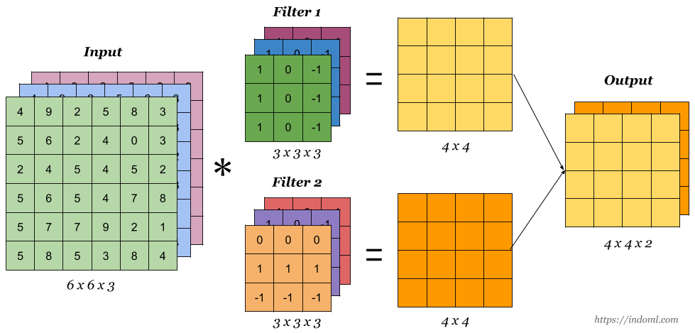
Convolutional layers are comprised of filters and feature maps. The filters are essentially the neurons of the layer. They have the weights and produce the input for the next layer. The feature map is the output of one filter applied to the previous layer.

Convolutions operate over 3D tensors, called feature maps, with two spatial axes (height and width) as well as a depth axis (also called the channels axis). For an RGB image, the dimension of the depth axis is 3, because the image has three color channels: red, green, and blue. For a black-and-white picture, like the MNIST digits, the depth is 1 (levels of gray). The convolution operation extracts patches from its input feature map and applies the same transformation to all of these patches, producing an output feature map. This output feature map is still a 3D tensor: it has a width and a height. Its depth can be arbitrary, because the output depth is a parameter of the layer, and the different channels in that depth axis no longer stand for specific colors as in RGB input; rather, they stand for filters. Filters encode specific aspects of the input data: at a high level, a single filter could encode the concept “presence of a face in the input,” for instance.

In the MNIST example that we will see, the first convolution layer takes a feature map of size (28, 28, 1) and outputs a feature map of size (26, 26, 32): it computes 32 filters over its input. Each of these 32 output channels contains a 26×26 grid of values, which is a response map of the filter over the input, indicating the response of that filter pattern at different locations in the input.

Convolutions are defined by two key parameters:

• Size of the patches extracted from the inputs. These are typically 3×3 or 5×5
• The number of filters computed by the convolution.

Padding: One of "valid", "causal" or "same" (case-insensitive). "valid" means "no padding". "same" results in padding the input such that the output has the same length as the original input. "causal" results in causal (dilated) convolutions,

1D Convolutional Network¶

In tf.keras see 1D convolutional layers

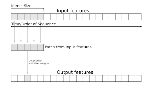
image source: Deep Learning with Python by François Chollet

2D Convolutional Network¶

In tf.keras see 2D convolutional layers

keras.layers.Conv2D (filters, kernel_size, strides=(1, 1), padding='valid', activation=None, use_bias=True, kernel_initializer='glorot_uniform', data_format='channels_last', bias_initializer='zeros')

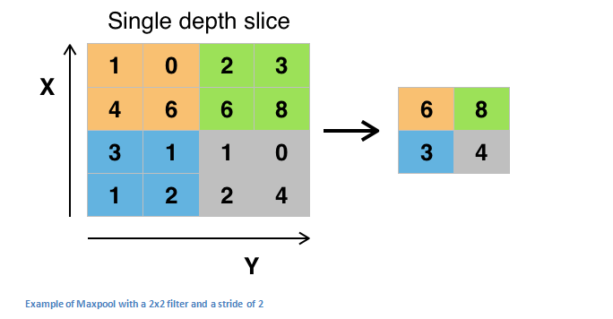
b. Pooling Layers.¶

Pooling layers are also comprised of filters and feature maps. Let's say the pooling layer has a 2x2 receptive field and a stride of 2. This stride results in feature maps that are one half the size of the input feature maps. We can use a max() operation for each receptive field.

In tf.keras see 2D pooling layers

keras.layers.MaxPooling2D(pool_size=(2, 2), strides=None, padding='valid', data_format=None)

c. Dropout Layers.¶

Dropout consists in randomly setting a fraction rate of input units to 0 at each update during training time, which helps prevent overfitting.

In tf.keras see Dropout layers

tf.keras.layers.Dropout(rate, seed=None)

rate: float between 0 and 1. Fraction of the input units to drop.
seed: A Python integer to use as random seed.

References

Dropout: A Simple Way to Prevent Neural Networks from Overfitting

d. Fully Connected Layers.¶

A fully connected layer flattens the square feature map into a vector. Then we can use a sigmoid or softmax activation function to output probabilities of classes.

In tf.keras see Fully Connected layers

keras.layers.Dense(units, activation=None, use_bias=True, kernel_initializer='glorot_uniform', bias_initializer='zeros')

Part 2: Preprocessing the data¶

Visualizing the different channels¶

If you want to learn more: Image Processing with Python and Scipy

Part 3: Putting the Parts together to make a small ConvNet Model¶

Let's put all the parts together to make a convnet for classifying our good old MNIST digits.

Notice: These photos do not have a third dimention channel because they are B&W.;

The next step is to feed the last output tensor (of shape (3, 3, 64)) into a densely connected classifier network like those you’re already familiar with: a stack of Dense layers. These classifiers process vectors, which are 1D, whereas the output of the last conv layer is a 3D tensor. First we have to flatten the 3D outputs to 1D, and then add a few Dense layers on top.

Data Preprocessing : Meet the ImageDataGenerator class in keras¶

(keras ImageGenerator documentation)

The MNIST and other pre-loaded dataset are formatted in a way that is almost ready for feeding into the model. What about plain images? They should be formatted into appropriately preprocessed floating-point tensors before being fed into the network.

The Dogs vs. Cats dataset that you’ll use isn’t packaged with Keras. It was made available by Kaggle as part of a computer-vision competition in late 2013, back when convnets weren’t mainstream. The data has been downloaded for you from https://www.kaggle.com/c/dogs-vs-cats/data The pictures are medium-resolution color JPEGs.

So you do indeed have 2,000 training images, 1,000 validation images, and 1,000 test images. Each split contains the same number of samples from each class: this is a balanced binary-classification problem, which means classification accuracy will be an appropriate measure of success.

Why do we need an extra dimension here?

Building the network¶

For the compilation step, you’ll go with the RMSprop optimizer. Because you ended the network with a single sigmoid unit, you’ll use binary crossentropy as the loss.

The steps for getting it into the network are roughly as follows:

1. Read the picture files.
2. Convert the JPEG content to RGB grids of pixels.
3. Convert these into floating-point tensors.
4. Rescale the pixel values (between 0 and 255) to the [0, 1] interval (as you know, neural networks prefer to deal with small input values).

It may seem a bit daunting, but fortunately Keras has utilities to take care of these steps automatically with the class ImageDataGenerator, which lets you quickly set up Python generators that can automatically turn image files on disk into batches of preprocessed tensors. This is what you’ll use here.

Let’s look at the output of one of these generators: it yields batches of 150×150 RGB images (shape (20, 150, 150, 3)) and binary labels (shape (20,)). There are 20 samples in each batch (the batch size). Note that the generator yields these batches indefinitely: it loops endlessly over the images in the target folder. For this reason, you need to break the iteration loop at some point:

Let’s fit the model to the data using the generator. You do so using the .fit_generator method, the equivalent of .fit for data generators like this one. It expects as its first argument a Python generator that will yield batches of inputs and targets indefinitely, like this one does.

Because the data is being generated endlessly, the Keras model needs to know how many samples to draw from the generator before declaring an epoch over. This is the role of the steps_per_epoch argument: after having drawn steps_per_epoch batches from the generator—that is, after having run for steps_per_epoch gradient descent steps - the fitting process will go to the next epoch. In this case, batches are 20 samples, so it will take 100 batches until you see your target of 2,000 samples.

When using fit_generator, you can pass a validation_data argument, much as with the fit method. It’s important to note that this argument is allowed to be a data generator, but it could also be a tuple of Numpy arrays. If you pass a generator as validation_data, then this generator is expected to yield batches of validation data endlessly; thus you should also specify the validation_steps argument, which tells the process how many batches to draw from the validation generator for evaluation

Let’s plot the loss and accuracy of the model over the training and validation data during training:

Let's try data augmentation

These are just a few of the options available (for more, see the Keras documentation). Let’s quickly go over this code:

• rotation_range is a value in degrees (0–180), a range within which to randomly rotate pictures.
• width_shift and height_shift are ranges (as a fraction of total width or height) within which to randomly translate pictures vertically or horizontally.
• shear_range is for randomly applying shearing transformations.
• zoom_range is for randomly zooming inside pictures.
• horizontal_flip is for randomly flipping half the images horizontally—relevant when there are no assumptions of - horizontal asymmetry (for example, real-world pictures).
• fill_mode is the strategy used for filling in newly created pixels, which can appear after a rotation or a width/height shift.

Let’s look at the augmented images

If you train a new network using this data-augmentation configuration, the network will never see the same input twice. But the inputs it sees are still heavily intercorrelated, because they come from a small number of original images—you can’t produce new information, you can only remix existing information. As such, this may not be enough to completely get rid of overfitting. To further fight overfitting, you’ll also add a Dropout layer to your model right before the densely connected classifier.

And let’s plot the results again. Thanks to data augmentation and dropout, you’re no longer overfitting: the training curves are closely tracking the validation curves. You now reach an accuracy of 82%, a 15% relative improvement over the non-regularized model. (Note: these numbers are for 100 epochs..)

By using regularization techniques even further, and by tuning the network’s parameters (such as the number of filters per convolution layer, or the number of layers in the network), you may be able to get an even better accuracy, likely up to 86% or 87%. But it would prove difficult to go any higher just by training your own convnet from scratch, because you have so little data to work with. As a next step to improve your accuracy on this problem, you’ll have to use a pretrained model.