CS109B Data Science 2: Advanced Topics in Data Science

Lab 4 - Bayesian Analysis¶

Harvard University
Spring 2020
Instructors: Mark Glickman, Pavlos Protopapas, and Chris Tanner
Lab Instructors: Chris Tanner and Eleni Angelaki Kaxiras
Content: Eleni Angelaki Kaxiras

---

Learning Objectives¶

By the end of this lab, you should be able to:

• Understand how probability distributions work.
• Apply Bayes Rule in calculating probabilities.
• Understand how to apply Bayesian analysis using PyMC3
• Avoid getting fired when talking to your Bayesian employer.

This lab corresponds to Lectures 6, 7, and 8, and maps to Homework 3.

Table of Contents¶

1. The Bayesian Way of Thinking or Is this a Fair Coin?
2. Intro to pyMC3.
3. Bayesian Linear Regression.
4. Try this at Home: Example on Mining Disasters.

1. The Bayesian way of Thinking¶

Here is my state of knowledge about the situation. Here is some data, I am now going to revise my state of knowledge.

A. Bayes Rule¶

\begin{equation} \label{eq:bayes} P(A|\textbf{B}) = \frac{P(\textbf{B} |A) P(A) }{P(\textbf{B})} \end{equation}

$P(A|\textbf{B})$ is the posterior distribution, prob(hypothesis | data)

$P(\textbf{B} |A)$ is the likelihood function, how probable is my data B for different values of the parameters

$P(A)$ is the marginal probability to observe the data, called the prior, this captures our belief about the data before observing it.

$P(\textbf{B})$ is the marginal distribution (sometimes called marginal likelihood)

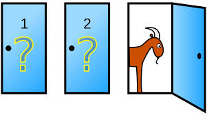
You are invited to play a game. There are 3 doors behind one of which are the keys to a brand new red Tesla. There is a goat behind each of the other two.

You are asked to pick one door, and let's say you pick Door1. The host knows where the keys are. Of the two remaining closed doors, he will always open the door that has a goat behind it. He'll say "I will do you a favor and open Door2". So he opens Door2 inside which there is, of course, a goat. He now asks you, do you want to open the initial Door you chose or change to Door3? Generally, in this game, when you are presented with this choice should you swap the doors?

Initial Steps:

• Start by defining the events of this probabilities game. One definition is:

  • $A_i$: car is behind door $i$

  • $B_i$ host opens door $i$

$i\in[1,2,3]$

• In more math terms, the question is: is the probability that the price is behind Door 1 higher than the probability that the price is behind Door2, given that an event has occured?

B. Bayes Rule written with Probability Distributions¶

We have data that we believe come from an underlying distribution of unknown parameters. If we find those parameters, we know everything about the process that generated this data and we can make inferences (create new data).

\begin{equation} \label{eq:bayes} P(\theta|\textbf{D}) = \frac{P(\textbf{D} |\theta) P(\theta) }{P(\textbf{D})} \end{equation}

But what is $\theta \;$?¶

$\theta$ is an unknown yet fixed set of parameters. In Bayesian inference we express our belief about what $\theta$ might be and instead of trying to guess $\theta$ exactly, we look for its probability distribution. What that means is that we are looking for the parameters of that distribution. For example, for a Poisson distribution our $\theta$ is only $\lambda$. In a normal distribution, our $\theta$ is often just $\mu$ and $\sigma$.

C. A review of Common Probability Distributions¶

Discrete Distributions¶

The random variable has a probability mass function (pmf) which measures the probability that our random variable will take a specific value $y$, denoted $P(Y=y)$.

• Bernoulli (binary outcome, success has probability $\theta$, $one$ trial): $ P(Y=k) = \theta^k(1-\theta)^{1-k} $

  ---

• Binomial (binary outcome, success has probability $\theta$, $n$ trials): \begin{equation} P(Y=k) = {{n}\choose{k}} \cdot \theta^k(1-\theta)^{n-k} \end{equation}

Note: Binomial(1,$p$) = Bernouli($p$)

---

• Negative Binomial

  ---

• Poisson (counts independent events occurring at a rate) \begin{equation} P\left( Y=y|\lambda \right) = \frac{{e^{ - \lambda } \lambda ^y }}{{y!}} \end{equation} y = 0,1,2,...

  ---

• Discrete Uniform

  ---

• Categorical, or Multinulli (random variables can take any of K possible categories, each having its own probability; this is a generalization of the Bernoulli distribution for a discrete variable with more than two possible outcomes, such as the roll of a die)

  ---

• Dirichlet-multinomial (a generalization of the beta distribution for many variables)

Continuous Distributions¶

The random variable has a probability density function (pdf).

• Uniform (variable equally likely to be near each value in interval $(a,b)$) \begin{equation} P(X = x) = \frac{1}{b - a} \end{equation} anywhere within the interval $(a, b)$, and zero elsewhere.

  ---

• Normal (a.k.a. Gaussian) \begin{equation} X \sim \mathcal{N}(\mu,\,\sigma^{2}) \end{equation}

  A Normal distribution can be parameterized either in terms of precision $\tau$ or standard deviation ($\sigma^{2}$. The link between the two is given by \begin{equation} \tau = \frac{1}{\sigma^{2}} \end{equation}

  • Mean $\mu$
  • Variance $\frac{1}{\tau}$ or $\sigma^{2}$
  • Parameters: mu: float, sigma: float or tau: float

    ---

• Beta (variable ($\theta$) taking on values in the interval $[0,1]$, and parametrized by two positive parameters, $\alpha$ and $\beta$ that control the shape of the distribution.

Note:Beta is a good distribution to use for priors (beliefs) because its range is $[0,1]$ which is the natural range for a probability and because we can model a wide range of functions by changing the $\alpha$ and $\beta$ parameters.

\begin{equation} \label{eq:beta} P(\theta) = \frac{1}{B(\alpha, \beta)} {\theta}^{\alpha - 1} (1 - \theta)^{\beta - 1} \propto {\theta}^{\alpha - 1} (1 - \theta)^{\beta - 1} \end{equation}

where the normalisation constant, $B$, is a beta function of $\alpha$ and $\beta$,

\begin{equation} B(\alpha, \beta) = \int_{t=0}^1 t^{\alpha - 1} (1 - t)^{\beta - 1} dt. \end{equation}

---

• Exponential

  ---

• Gamma

Code Resources:¶

• Statistical Distributions in numpy/scipy: scipy.stats
• Statistical Distributions in pyMC3: distributions in PyMC3 (we will see those below).

Change the value of $\mu$ in the Poisson PMF and see how the plot changes. Remember that the y-axis in a discrete probability distribution shows the probability of the random variable having a specific value in the x-axis.

\begin{equation} P\left( X=k \right) = \frac{{e^{ - \mu } \mu ^k }}{{k!}} \end{equation}

stats.poisson.pmf(x, mu) $\mu$(mu) is our $\theta$ in this case.

Change the value of $\mu$ in the Uniform PDF and see how the plot changes.

Remember that the y-axis in a continuous probability distribution does not shows the actual probability of the random variable having a specific value in the x-axis because that probability is zero!. Instead, to see the probability that the variable is within a small margin we look at the integral below the curve of the PDF.

The uniform is often used as a noninformative prior.

Uniform - numpy.random.uniform(a=0.0, b=1.0, size)

$\alpha$ and $\beta$ are our parameters. size is how many tries to perform. Our $\theta$ is basically the combination of the parameters a,b. We can also call it \begin{equation} \mu = (a+b)/2 \end{equation}

D. Is this a Fair Coin?¶

We do not want to promote gambling but let's say you visit the casino in Monte Carlo. You want to test your theory that casinos are dubious places where coins have been manipulated to have a larger probability for tails. So you will try to estimate how fair a coin is based on 100 flips.
You begin by flipping the coin. You get either Heads ($H$) or Tails ($T$) as our observed data and want to see if your posterior probabilities change as you obtain more data, that is, more coin flips. A nice way to visualize this is to plot the posterior probabilities as we observe more flips (data).

We will be using Bayes rule. $\textbf{D}$ is our data.

\begin{equation} \label{eq:bayes} P(\theta|\textbf{D}) = \frac{P(\textbf{D} |\theta) P(\theta) }{P(\textbf{D})} \end{equation}

In the case of a coin toss when we observe $k$ heads in $n$ tosses: \begin{equation} \label{eq:bayes} P(\theta|\textbf{k}) = Beta(\alpha + \textbf{k}, \beta + n - \textbf{k}) \end{equation}

we can say that $\alpha$ and $\beta$ play the roles of a "prior number of heads" and "prior number of tails".

Top

2. Introduction to pyMC3¶

PyMC3 is a Python library for programming Bayesian analysis, and more specifically, data creation, model definition, model fitting, and posterior analysis. It uses the concept of a model which contains assigned parametric statistical distributions to unknown quantities in the model. Within models we define random variables and their distributions. A distribution requires at least a name argument, and other parameters that define it. You may also use the logp() method in the model to build the model log-likelihood function. We define and fit the model.

PyMC3 includes a comprehensive set of pre-defined statistical distributions that can be used as model building blocks. Although they are not meant to be used outside of a model, you can invoke them by using the prefix pm, as in pm.Normal.

Markov Chain Monte Carlo (MCMC) Simulations¶

PyMC3 uses the No-U-Turn Sampler (NUTS) and the Random Walk Metropolis, two Markov chain Monte Carlo (MCMC) algorithms for sampling in posterior space. Monte Carlo gets into the name because when we sample in posterior space, we choose our next move via a pseudo-random process. NUTS is a sophisticated algorithm that can handle a large number of unknown (albeit continuous) variables.

References:

• Salvatier J, Wiecki TV, Fonnesbeck C. 2016. Probabilistic programming in Python using PyMC3. PeerJ Computer Science 2:e55 (https://doi.org/10.7717/peerj-cs.55)
• Distributions in PyMC3
• More Details on Distributions

Information about PyMC3 functions including descriptions of distributions, sampling methods, and other functions, is available via the help command.

Top

3. Bayesian Linear Regression¶

Let's say we want to predict outcomes Y as normally distributed observations with an expected value $mu$ that is a linear function of two predictor variables, $\bf{x}_1$ and $\bf{x}_2$.

\begin{equation} \mu = \alpha + \beta_1 \bf{x}_1 + \beta_2 x_2 \end{equation}\begin{equation} Y \sim \mathcal{N}(\mu,\,\sigma^{2}) \end{equation}

where $\sigma^2$ represents the measurement error.

In this example, we will use $\sigma^2 = 10$

We also choose the parameters as normal distributions:

\begin{eqnarray} \alpha \sim \mathcal{N}(0,\,10) \\ \beta_i \sim \mathcal{N}(0,\,10) \\ \sigma^2 \sim |\mathcal{N}(0,\,10)| \end{eqnarray}

We will artificially create the data to predict on. We will then see if our model predicts them correctly.

This linear regression example is from the original paper on PyMC3: Salvatier J, Wiecki TV, Fonnesbeck C. 2016. Probabilistic programming in Python using PyMC3. PeerJ Computer Science 2:e55 https://doi.org/10.7717/peerj-cs.55

Top

4. Try this at Home: Example on Mining Disasters¶

We will go over the classical mining disasters from 1851 to 1962 dataset.

This example is from the pyMC3 Docs.

Building the model¶

Step1: We choose the probability model for our experiment. Occurrences of disasters in the time series is thought to follow a Poisson process with a large rate parameter in the early part of the time series, and from one with a smaller rate in the later part. We are interested in locating the change point in the series, which perhaps is related to changes in mining safety regulations.

disasters = pm.Poisson('disasters', rate, observed=disaster_data)

We have two rates, early_rate if $t<=s$, and late_rate if $t>s$, where $s$ is the year the switch was made (a.k.a. the switchpoint).

Step2: Choose a prior distributions of the two rates, what we believe the rates were before we observed the data, and the switchpoint. We choose Exponential.

early_rate = pm.Exponential('early_rate', 1)

The parameters of this model are:

Note: Watch for missing values. Missing values are handled transparently by passing a MaskedArray or a pandas.DataFrame. Behind the scenes, another random variable, disasters.missing_values is created to model the missing values. If you pass a np.array with missing values you will get an error.

Model Fitting¶

Posterior Analysis¶

On the left side plots we notice that our early rate is between 2.5 and 3.5 disasters a year. In the late period it seems to be between 0.6 and 1.2 so definitely lower.

The right side plots show the samples we drew to come to our conclusion.