{
"cells": [
{
"cell_type": "markdown",
"metadata": {},
"source": [
"# Title\n",
"\n",
"**Exercise - Multi-class Classification and PCA**\n",
"\n",
"# Description\n",
"\n",
"This exercise follows more like a lab and is broken into 3 parts (we will reconvene after each part). The 3 parts are:\n",
"1. Data set exploration and baseline models (graded)\n",
"2. PCA and PCR (graded)\n",
"3. Going Further with the dataset (not graded)\n",
"\n",
"# Learning Goals\n",
"\n",
"In this lab, we will look at how to use PCA to reduce a dataset to a smaller number of dimensions. The goals are:\n",
"- Better Understand the multiclass setting\n",
"- Understand what PCA is and why it's useful\n",
"- Feel comfortable performing PCA on a new dataset\n",
"- Understand what it means for each component to capture variance from the original dataset\n",
"- Be able to extract the `variance explained` by components\n",
"- Perform modeling with the PCA components\n",
"\n",
"# Hints:\n",
"\n",
"sklearn.accuracy_score : Generates a Logistic Regression Model\n",
"\n",
"sklearn.LogisticRegression : Generates a Logistic Regression Model\n",
"\n",
"sklearn.LogisticRegressionCV : Uses CV to perform regularization in Logistic Regression\n",
"\n",
"sklearn.PCA : Create a Principal Component Analysis (PCA) decomposition\n",
"\n",
"**Note: This exercise is auto-graded and you can try multiple attempts.**"
]
},
{
"cell_type": "markdown",
"metadata": {},
"source": [
"#  CS-109A Introduction to Data Science\n",
"\n",
"\n",
"## Lecture 21: More on Classification and PCA\n",
"\n",
"**Harvard University**
CS-109A Introduction to Data Science\n",
"\n",
"\n",
"## Lecture 21: More on Classification and PCA\n",
"\n",
"**Harvard University**
\n",
"**Fall 2020**
\n",
"**Instructors:** Pavlos Protopapas, Kevin Rader, Chris Tanner
\n",
"**Contributors:** Kevin Rader, Eleni Kaxiras, Chris Tanner, Will Claybaugh, David Sondak\n",
"\n",
"---"
]
},
{
"cell_type": "code",
"execution_count": 1,
"metadata": {},
"outputs": [],
"source": [
"## RUN THIS CELL TO PROPERLY HIGHLIGHT THE EXERCISES\n",
"import requests\n",
"from IPython.core.display import HTML\n",
"styles = requests.get(\"https://raw.githubusercontent.com/Harvard-IACS/2018-CS109A/master/content/styles/cs109.css\").text\n",
"HTML(styles)"
]
},
{
"cell_type": "markdown",
"metadata": {},
"source": [
"## Learning Goals\n",
"In this lab, we will look at how to use PCA to reduce a dataset to a smaller number of dimensions. The goals are:\n",
"\n",
" - Better Understand the multiclass setting
\n",
" - Understand what PCA is and why it's useful
\n",
" - Feel comfortable performing PCA on a new dataset
\n",
" - Understand what it means for each component to capture variance from the original dataset
\n",
" - Be able to extract the `variance explained` by components
\n",
" - Perform modelling with the PCA components
\n",
"
"
]
},
{
"cell_type": "code",
"execution_count": 25,
"metadata": {},
"outputs": [],
"source": [
"%matplotlib inline\n",
"import numpy as np\n",
"import scipy as sp\n",
"import matplotlib.pyplot as plt\n",
"import seaborn as sns\n",
"import pandas as pd\n",
"\n",
"from sklearn.linear_model import LogisticRegressionCV\n",
"from sklearn.linear_model import LassoCV\n",
"from sklearn.metrics import accuracy_score\n",
"pd.set_option('display.width', 500)\n",
"pd.set_option('display.max_columns', 100)\n",
"pd.set_option('display.notebook_repr_html', True)\n",
"\n",
"from sklearn.model_selection import train_test_split"
]
},
{
"cell_type": "markdown",
"metadata": {},
"source": [
"## Part 0: Introduction\n",
"\n",
"What is PCA? PCA is a deterministic technique to transform data to a lowered dimensionality, whereby each feature/dimension captures the most variance possible.\n",
"\n",
"Why do we care to use it?\n",
"\n",
" - Visualizating the components can be useful
\n",
" - Allows for more efficient use of resources (time, memory)
\n",
" - Statistical reasons: fewer dimensions -> better generalization
\n",
" - noise removal / collinearity (improving data quality)
\n",
"
\n",
"\n",
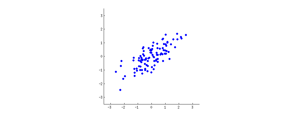
"Imagine some dataset where we have two features that are pretty redundant. For example, maybe we have data concerning elite runners. Two of the features may include ``VO2 max`` and ``heartrate``. These are highly correlated. We probably don't need both, as they don't offer much additional information from each other. Using a [great visual example from online](https://stats.stackexchange.com/questions/2691/making-sense-of-principal-component-analysis-eigenvectors-eigenvalues), let's say that this unlabelled graph **(always label your axis)** represents those two features:\n",
"\n",
"\n",
"\n",
"Let's say that this is our entire dataset, just 2 dimensions. If we wish to reduce the dimensions, we can only reduce it to just 1 dimension. A straight line is just 1 dimension (to help clarify this: imagine your straight line as being the x-axis, and values can be somewhere on this axis, but that's it. There is no y-axis dimension for a straight line). So, how should PCA select a straight line through this data?\n",
"\n",
"Below, the image shows all possible projects that are centered in the data:\n",
"\n",
"\n",
"\n",
"PCA picks the line that:\n",
"\n",
"- captures the most variance possible
\n",
"- minimizes the distance of the transformed points (distance from the original to the new space)
\n",
"
\n",
"\n",
"The animation **suggests** that these two aspects are actually the same. In fact, this is objectively true, but the proof for which is beyond the scope of the material for now. Feel free to read more at [this explanation](https://stats.stackexchange.com/questions/32174/pca-objective-function-what-is-the-connection-between-maximizing-variance-and-m/136072#136072) and via [Andrew Ng's notes](http://cs229.stanford.edu/notes/cs229-notes-all/cs229-notes10.pdf).\n",
"\n",
"In short, PCA is a math technique that works with the covariance matrix -- the matrix that describes how all pairwise features are correlated with one another. Covariance of two variables measures the degree to which they moved/vary in the same directin; how much one variable affects the other. A positive covariance means they are positively related (i.e., x1 increases as x2 does); negative means negative correlation (x1 decreases as x2 increases).\n",
"\n",
"In data science and machine learning, our models are often just finding patterns in the data this is easier if the data is spread out across each dimension and for the data features to be independent from one another (imagine if there's no variance at all. We couldn't do anything). Can we transform the data into a new set that is a linear combination of those original features?\n",
"\n",
"PCA finds new dimensions (set of basis vectors) such that all the dimensions are orthogonal and hence linearly independent, and ranked according to the variance (eigenvalue). That is, the first component is the most important, as it captures the most variance."
]
},
{
"cell_type": "markdown",
"metadata": {},
"source": [
"---"
]
},
{
"cell_type": "markdown",
"metadata": {},
"source": [
"## Part 1a: The Wine Quality Dataset\n",
"\n",
"Imagine that a wine sommelier has tasted and rated 1,000 distinct wines, and now that she's highly experienced, she is curious if she can more efficiently rate wines without even trying them. That is, perhaps her tasting preferences follow a pattern, allowing her to predict the rating a new wine without even trying it! \n",
"\n",
"The dataset contains 11 chemical features, along with a quality scale from 1-10; however, only values of 3-9 are actually used in the data. The ever-elusive perfect wine has yet to be tasted. \n",
"\n",
"#### **NOTE:** While this dataset involves the topic of alcohol, we, the CS109A staff, along with Harvard at large is in no way encouraging alcohol use, and this example should not be intrepreted as any endorsement for such; it is merely a pedagogical example. I apologize if this example offends anyone or is off-putting.\n",
"\n"
]
},
{
"cell_type": "markdown",
"metadata": {},
"source": [
"### Read-in and checking\n",
"First, let's read-in the data and verify it:"
]
},
{
"cell_type": "code",
"execution_count": 61,
"metadata": {},
"outputs": [],
"source": [
"wines_df = pd.read_csv(\"data/wines.csv\")\n",
"wines_df.head()"
]
},
{
"cell_type": "code",
"execution_count": 62,
"metadata": {},
"outputs": [],
"source": [
"wines_df.describe()"
]
},
{
"cell_type": "markdown",
"metadata": {},
"source": [
"For this exercise, let's say that the wine expert is curious if she can predict, as a rough approximation, the **categorical quality -- bad, average, or great.** Let's define those categories as follows:\n",
"\n",
"- `bad` is when for wines that have a quality <= 5\n",
"- `average` is when a wine has a quality of 6\n",
"- `great` is when a wine has a quality of >= 7"
]
},
{
"cell_type": "markdown",
"metadata": {},
"source": [
"**Q1.1** For sanity, let's see how many wines will end up in each quality category (create the barplot)"
]
},
{
"cell_type": "code",
"execution_count": 63,
"metadata": {},
"outputs": [],
"source": [
"counts = np.unique(wines_df['quality'],return_counts=True)\n",
"\n",
"### use seaborn to create a barplot\n",
"sns.barplot(x=___,y=___);"
]
},
{
"cell_type": "code",
"execution_count": 64,
"metadata": {},
"outputs": [],
"source": [
"##### copy the original data so that we're free to make changes\n",
"wines_df_recode = wines_df.copy()\n",
"\n",
"# use the 'cut' function to reduce a variable down to the aforementioned bins (inclusive boundaries)\n",
"wines_df_recode['quality'] = pd.cut(wines_df_recode['quality'],[0,5,6,10], labels=[0,1,2])\n",
"wines_df_recode.loc[wines_df_recode['quality'] == 1]\n",
"\n",
"# drop the un-needed columns\n",
"x_data = wines_df_recode.drop(['quality'], axis=1)\n",
"y_data = wines_df_recode['quality']\n",
"\n",
"x_train, x_test, y_train, y_test = train_test_split(x_data, y_data, test_size=.2, random_state=8, stratify=y_data)\n",
"\n",
"# previews our data to check if we correctly constructed the labels (we did)\n",
"print(wines_df['quality'].head())\n",
"print(wines_df_recode['quality'].head())"
]
},
{
"cell_type": "code",
"execution_count": 65,
"metadata": {},
"outputs": [],
"source": [
"y_data.value_counts()\n"
]
},
{
"cell_type": "markdown",
"metadata": {},
"source": [
"Now that we've split the data, let's look to see if there are any obvious patterns (correlations between different variables)."
]
},
{
"cell_type": "code",
"execution_count": 66,
"metadata": {},
"outputs": [],
"source": [
"from pandas.plotting import scatter_matrix\n",
"scatter_matrix(wines_df_recode, figsize=(30,20));"
]
},
{
"cell_type": "markdown",
"metadata": {},
"source": [
"It looks like there aren't any particularly strong correlations among the predictors (maybe `total sulfur dioxide` and `free sulfur dioxide`) so we're safe to keep them all.\n",
"\n",
"## Part 1b: Baseline Prediction Models\n",
"Before we do anything too fancy, it's always best to start with something simple.\n",
"\n",
"### Baseline\n",
"The baseline estimate is barely a model -- it simple returns the single label/class occurs the most often (in the training data). In other words, whichever label/class is most popular, it will always preduct that as its answer, completely independent of any x-data. Above, we saw that the most popular label was `average`, represented by 432 of our 1,000 wines. Thus, our MLE should yield `average` for all inputs:"
]
},
{
"cell_type": "code",
"execution_count": 67,
"metadata": {},
"outputs": [],
"source": [
"baseline_class = y_data.value_counts().idxmax()\n",
"baseline_train_accuracy = len(y_train.loc[y_train == baseline_class]) / len(y_train)\n",
"baseline_test_accuracy = len(y_test.loc[y_test == baseline_class]) / len(y_test)\n",
"\n",
"\n",
"scores = [[baseline_train_accuracy, baseline_test_accuracy]]\n",
"names = ['baseline']\n",
"df_results = pd.DataFrame(scores, index=names, columns=['Train Accuracy', 'Test Accuracy'])\n",
"df_results"
]
},
{
"cell_type": "markdown",
"metadata": {},
"source": [
"Baseline gives a predictive accuracy is **43.3%** on the test set. Hopefully we can do better than this."
]
},
{
"cell_type": "markdown",
"metadata": {},
"source": [
"### Logistic Regression\n",
"Logistic regression is used for predicting categorical outputs, which is exactly what our task concerns. So, let's create a multiclass logistic regression model (`ovr`: one-vs.-rest):"
]
},
{
"cell_type": "code",
"execution_count": 68,
"metadata": {
"scrolled": true
},
"outputs": [],
"source": [
"from sklearn.linear_model import LogisticRegression\n",
"lr = LogisticRegression(C=1000000, solver='lbfgs', multi_class='ovr', max_iter=10000).fit(x_train,y_train)\n",
"print(\"Coefficients:\", lr.coef_)\n",
"print(\"Intercepts:\", lr.intercept_)"
]
},
{
"cell_type": "markdown",
"metadata": {},
"source": [
"**Q1.2** What is stored in `.coef_` and `.intercept_`? Why are there so many of them?\n"
]
},
{
"cell_type": "markdown",
"metadata": {},
"source": [
"*your answer here*"
]
},
{
"cell_type": "markdown",
"metadata": {},
"source": [
"**Q1.3** Determine measure its performance as measured by classific ation accuracy:"
]
},
{
"cell_type": "code",
"execution_count": 69,
"metadata": {},
"outputs": [],
"source": [
"### edTest(test_acc) ###\n",
"\n",
"lr_train_accuracy = lr.score(___,___)\n",
"lr_test_accuracy = lr.score(___,___)\n",
"\n",
"# appends results to our dataframe\n",
"names.append('Logistic Regression')\n",
"scores.append([lr_train_accuracy, lr_test_accuracy])\n",
"df_results = pd.DataFrame(scores, index=names, columns=['Train Accuracy', 'Test Accuracy'])\n",
"df_results"
]
},
{
"cell_type": "markdown",
"metadata": {},
"source": [
"Yay, that's better than our baseline performance. Can we do better with cross-validation?\n",
"\n",
"## Part 1c: Tuning our Prediction Model\n",
"\n",
"#### Summary\n",
"- Logistic regression extends OLS to work naturally with a dependent variable that's only ever 0 and 1.\n",
"- In fact, Logistic regression is even more general and is used for predicting the probability of an example belonging to each of $N$ classes.\n",
"- The code for the two cases is identical and just like `LinearRegression`: `.fit`, `.score`, and all the rest\n",
"- Significant predictors does not imply that the model actually works well. Signifigance can be driven by data size alone.\n",
"- The data aren't enough to do what we want\n",
"\n",
"**Warning**: Logistic regression _tries_ to hand back valid probabilities. As with all models, you can't trust the results until you validate them- if you're going to use raw probabilities instead of just predicted class, take the time to verify that if you pool all cases where the model says \"I'm 30% confident it's class A\" 30% of them actually are class A."
]
},
{
"cell_type": "markdown",
"metadata": {},
"source": [
"**Q1.4** Use `LogisticRegressionCV` to build a better tuned `ovr` (lasso-based) model based on all of these predictors."
]
},
{
"cell_type": "code",
"execution_count": 70,
"metadata": {},
"outputs": [],
"source": [
"### edTest(test_logitCV) ###\n",
"\n",
"logit_regr_lasso = LogisticRegressionCV(solver='liblinear', multi_class=___, penalty=___, max_iter=___, cv=10)\n",
"logit_regr_lasso.fit(x_train,y_train) # fit\n",
"\n",
"y_train_pred_lasso = ___ # predict the test set\n",
"y_test_pred_lasso = ___ # predict the test set\n",
"\n",
"train_score_lasso = ___ # get train accuracy\n",
"test_score_lasso = ___ # get test accuracy\n",
"\n",
"names.append('Logistic Regression w/ CV + Lasso')\n",
"scores.append([train_score_lasso, test_score_lasso])\n",
"df_results = pd.DataFrame(scores, index=names, columns=['Train Accuracy', 'Test Accuracy'])\n",
"df_results"
]
},
{
"cell_type": "markdown",
"metadata": {},
"source": [
"**Q1.5**: Hmm, cross-validation didn't seem to offer much improved results. Is this correct? Is it possible for cross-validation to not yield much better results than non-cross-validation? If so, why is that happening here? What else should we consider?\n"
]
},
{
"cell_type": "markdown",
"metadata": {},
"source": [
"*your answer here*"
]
},
{
"cell_type": "markdown",
"metadata": {},
"source": [
"---"
]
},
{
"cell_type": "markdown",
"metadata": {},
"source": [
"## Part 2: Dimensionality Reduction\n",
"In attempt to improve performance, we may wonder if some of our features are redundant and are posing difficulties for our logistic regression model. \n",
"\n",
"**Q2.1**: Let's PCA decompose our predictors to shrink the problem down to 2 dimensions (with as little loss as possible) and see if that gives us a clue about what makes this problem tough."
]
},
{
"cell_type": "code",
"execution_count": 50,
"metadata": {
"scrolled": true
},
"outputs": [],
"source": [
"from sklearn.decomposition import PCA\n",
"from sklearn.preprocessing import StandardScaler\n",
"\n",
"num_components = 2\n",
"\n",
"# scale the datasets\n",
"scale_transformer = StandardScaler(copy=True).fit(x_train)\n",
"x_train_scaled = scale_transformer.transform(x_train)\n",
"x_test_scaled = scale_transformer.transform(x_test)\n",
"\n",
"# reduce dimensions\n",
"pca_transformer = PCA(___).fit(___)\n",
"x_train_2d = pca_transformer.transform(___)\n",
"x_test_2d = pca_transformer.transform(___)\n",
"\n",
"print(x_train_2d.shape)\n",
"x_train_2d[0:5,:]"
]
},
{
"cell_type": "markdown",
"metadata": {},
"source": [
"**NOTE:**\n",
"1. Both scaling and reducing dimension follow the same pattern: we fit the object to the training data, then use .transform() to convert the training and test data. This ensures that, for instance, we scale the test data using the _training_ mean and variance, not its own mean and variance\n",
"2. We need to equalize the variance of each feature before applying PCA; otherwise, certain dimensions will dominate the scaling. Our PCA dimensions would just be the features with the largest spread."
]
},
{
"cell_type": "markdown",
"metadata": {},
"source": [
"**Q2.2**: Why didn't we scale the y-values (class labels) or transform them with PCA? Is this a mistake?\n"
]
},
{
"cell_type": "markdown",
"metadata": {},
"source": [
"*your answer here*"
]
},
{
"cell_type": "markdown",
"metadata": {},
"source": [
"**Q2.3**: Our data only has 2 dimensions/features now. What do these features represent?"
]
},
{
"cell_type": "code",
"execution_count": 52,
"metadata": {},
"outputs": [],
"source": [
"# your code here "
]
},
{
"cell_type": "markdown",
"metadata": {},
"source": [
"*your answer here*"
]
},
{
"cell_type": "markdown",
"metadata": {},
"source": [
"Since our data only has 2 dimensions now, we can easily visualize the entire dataset. If we choose to color each datum with respect to its associated label/class, it allows us to see how separable the data is. That is, it gives an indication as to how easy/difficult it is for a model to fit the new, transformed data.\n",
"\n",
"**Q2.4**: Create the scatterplot with color-coded points for the 3 classes of wine quaslity, and put PCA vector 1 on the x-axis and PCA vector 2 on the y-axis."
]
},
{
"cell_type": "code",
"execution_count": 53,
"metadata": {},
"outputs": [],
"source": [
"# notice that we set up lists to track each group's plotting color and label\n",
"colors = ['r','c','b']\n",
"label_text = [\"Bad Wines\", \"Average Wines\", \"Great Wines\"]\n",
"\n",
"# and we loop over the different groups\n",
"for cur_quality in [0,1,2]:\n",
" cur_df = x_train_2d[y_train==cur_quality]\n",
" plt.scatter(___, ___, c = colors[cur_quality], label=label_text[cur_quality])\n",
"\n",
"# all plots need labels\n",
"plt.xlabel(\"PCA Dimension 1\")\n",
"plt.ylabel(\"PCA Dimention 2\")\n",
"plt.legend();"
]
},
{
"cell_type": "markdown",
"metadata": {},
"source": [
"Well, that gives us some idea of why the problem is difficult! The bad, average, and great wines are all on top of one another. Not only are there few great wines, which we knew from the beginning, but there is no line that can easily separate the classes of wines."
]
},
{
"cell_type": "markdown",
"metadata": {},
"source": [
"**Q2.5**: \n",
"\n",
"\n",
" - What critique can you make against the plot above? Why does this plot not prove that the different wines are hopelessly similar?
\n",
" - The wine data we've used so far consist entirely of continuous predictors. Would PCA work with categorical data?
\n",
"- Looking at our PCA plot above, we see something peculiar: we have two disjoint clusters, both of which have immense overlap in the qualities of wines.What could cause this? What does this mean?
\n",
"
\n"
]
},
{
"cell_type": "markdown",
"metadata": {},
"source": [
"*your answer here*"
]
},
{
"cell_type": "markdown",
"metadata": {},
"source": [
"Let's plot the same PCA'd data, but let's color code them according to if the wine is red or white"
]
},
{
"cell_type": "code",
"execution_count": 56,
"metadata": {},
"outputs": [],
"source": [
"# notice that we set up lists to track each group's plotting color and label\n",
"colors = ['r','c','b']\n",
"label_text = [\"Reds\", \"Whites\"]\n",
"\n",
"# and we loop over the different groups\n",
"for cur_color in [0,1]:\n",
" cur_df = x_train_2d[x_train['red']==cur_color]\n",
" plt.scatter(___, ___, c = colors[cur_color], label=label_text[cur_color])\n",
" \n",
"# all plots need labels\n",
"plt.xlabel(\"PCA Dimension 1\")\n",
"plt.ylabel(\"PCA Dimention 2\")\n",
"plt.legend();"
]
},
{
"cell_type": "markdown",
"metadata": {},
"source": [
"**Q2.6**: Wow. Look at that separation. Too bad we aren't trying to predict if a wine is red or white. Does this graph help you answer our previous question? Does it change your thoughts?\n"
]
},
{
"cell_type": "markdown",
"metadata": {},
"source": [
"*your answer here*"
]
},
{
"cell_type": "markdown",
"metadata": {},
"source": [
"## Part 2b. Evaluating PCA: Variance Explained and Predictions\n",
"One of the criticisms we made of the PCA plot was that it's lost something from the original data. Heck, we're only using 2 dimensions, we it's perfectly reasonable and expected for us to lose some information -- our goal was that the information we were discarding was noise.\n",
"\n",
"Let's investigate how much of the original data's structure the 2-D PCA captures. We'll look at the `explained_variance_ratio_` portion of the PCA fit. This lists, in order, the percentage of the x data's total variance that is captured by the nth PCA dimension."
]
},
{
"cell_type": "code",
"execution_count": 58,
"metadata": {},
"outputs": [],
"source": [
"var_explained = pca_transformer.explained_variance_ratio_\n",
"print(\"Variance explained by each PCA component:\", var_explained)\n",
"print(\"Total Variance Explained:\", np.sum(var_explained))"
]
},
{
"cell_type": "markdown",
"metadata": {},
"source": [
"The first PCA dimension captures 33% of the variance in the data, and the second PCA dimension adds another 20%. Together, we've captured about half of the total variation in the training data with just these two dimensions. So far, we've used PCA to transform our data, we've visualized our newly transformed data, and we've looked at the variance that it captures from the original dataset. That's a good amount of inspection; now let's actually use our transformed data to make predictions.\n",
"\n",
"
\n",
"\n",
"**Q2.7** Use Logistic Regression (with and without cross-validation) on the PCA-transformed data. Do you expect this to outperform our original accuracy? What are your results? Does this seem reasonable?"
]
},
{
"cell_type": "code",
"execution_count": 59,
"metadata": {},
"outputs": [],
"source": [
"### edTest(test_lrPCA) ###\n",
"\n",
"# do the non-CV approach here (create CV on your own if you'd like)\n",
"lr_pca = ___\n",
"\n",
"lr_pca_train_accuracy = ___\n",
"lr_pca_test_accuracy = ___\n",
"\n",
"names.append('Logistic Regression w/ PCA')\n",
"___\n",
"___\n",
"df_results"
]
},
{
"cell_type": "markdown",
"metadata": {},
"source": [
"We're only using 2 dimensions. What if we increase our data to the full PCA components?"
]
},
{
"cell_type": "markdown",
"metadata": {},
"source": [
"**Q2.8**: How can we incorporate the type of wine (Red vs. White) into this analysis (hink of at least 2 different approaches)? Can these both approaches be used for the PCA and non-PCA models?"
]
},
{
"cell_type": "markdown",
"metadata": {},
"source": []
},
{
"cell_type": "markdown",
"metadata": {},
"source": [
"---"
]
},
{
"cell_type": "markdown",
"metadata": {},
"source": [
"## Part 3: Going further with PCA\n",
"\n",
"**Q3.1**:\n",
" Fit a PCA that finds the complete PCA decomposition of our training data predictors\n",
" Use `np.cumsum()` to print out the variance we'd be able to explain by using n PCA dimensions for all choices of components.\n",
" Does the full-dimension PCA agree with the 2d PCA on how much variance the first components explain? **Do the full and 2d PCAs find the same first two dimensions? Why or why not?**\n",
" Make a plot of number of PCA dimensions against total variance explained. What PCA dimension looks good to you?\n",
" Use cross-validation to determine how many of the PCA copmonents add to the predictive nature of the PCR. \n",
"\n",
"Hint: `np.cumsum` stands for 'cumulative sum', so `np.cumsum([1,3,2,-1,2])` is `[1,4,6,5,7]`"
]
},
{
"cell_type": "code",
"execution_count": 60,
"metadata": {},
"outputs": [],
"source": [
"#your code here"
]
},
{
"cell_type": "markdown",
"metadata": {},
"source": [
"The plot above can be used to inform of us when we reach diminishing returns on variance explained. That is, the 'elbow' of the line is probably an ideal number of dimensions to use, at least with respect to the amount of variance explained.\n",
"\n",
"
\n",
"\n",
"**Q3.2** Looking at your graph, what is the 'elbow' point / how many PCA components do you think we should use? Does this number of components agree with the cross-validated predictive performance of the PCR? Explain."
]
},
{
"cell_type": "markdown",
"metadata": {},
"source": [
"*your answer here*"
]
},
{
"cell_type": "markdown",
"metadata": {},
"source": [
"## Part 3b: PCA Debriefing:\n",
"\n",
"- PCA maps a high-dimensional space into a lower dimensional space.\n",
"- The PCA dimensions are ordered by how much of the original data's variance they capture\n",
" - There are other cool and useful properties of the PCA dimensions (orthogonal, etc.). See a [textbook](http://math.mit.edu/~gs/linearalgebra/).\n",
"- PCA on a given dataset always gives the same dimensions in the same order.\n",
"- You can select the number of dimensions by fitting a big PCA and examining a plot of the cumulative variance explained.\n",
"\n",
"PCA is not guaranteed to improve predictive performance at all. As you've learned in class now, none of our models are guaranteed to always outperform others on all datasets; analyses are a roll of the dice. The goal is to have a suite of tools to allow us to gather, process, disect, model, and visualize the data -- and to learn which tools are better suited to which conditions. Sometimes our data isn't the most conducive to certain tools, and that's okay.\n",
"\n",
"What can we do about it?\n",
"1. Be honest about the methods and the null result. Lots of analyses fail.\n",
"2. Collect a dataset you think has a better chance of success. Maybe we collected the wrong chemical signals...\n",
"3. Keep trying new approaches. Just beware of overfitting the data you're validating on. Always have a test set locked away for when the final model is built.\n",
"4. Change the question. Maybe something you noticed during analysis seems interesting or useful (classifying red versus white). But again, you the more you try, the more you might overfit, so have test data locked away.\n",
"5. Just move on. If the odds of success start to seem small, maybe you need a new project."
]
},
{
"cell_type": "code",
"execution_count": null,
"metadata": {},
"outputs": [],
"source": []
},
{
"cell_type": "markdown",
"metadata": {},
"source": [
"---"
]
}
],
"metadata": {
"kernelspec": {
"display_name": "Python 3",
"language": "python",
"name": "python3"
},
"language_info": {
"codemirror_mode": {
"name": "ipython",
"version": 3
},
"file_extension": ".py",
"mimetype": "text/x-python",
"name": "python",
"nbconvert_exporter": "python",
"pygments_lexer": "ipython3",
"version": "3.8.5"
}
},
"nbformat": 4,
"nbformat_minor": 4
}