Key Word(s): Dask, Python, Parallel Computing
 AC295: Advanced Practical Data Science
Lecture 4: Dask
Harvard University
Spring 2020
Instructors: Pavlos Protopapas
TF: Michael Emanuel, Andrea Porelli and Giulia Zerbini
Author: Andrea Porelli and Pavlos Protopapas
Part 1: Scalable computing
1.1 Dask API
- what makes it unique:
- allows to work with larger datasets making it possible to parallelize computation
- it is helpful when size increases and even when "simple" sorting and aggregating would otherwise spill on persistent memory
- it simplifies the cost of using more complex infrastructure
- it is easy to learn for data scientists with a background in the Python (similar syntax) and flexible
- it helps applying distributed computing to data science project:
- not of great help for small size datasets: complex operations can be done without spilling to disk and slowing down process. Actually it would generate greater overheads.
- very useful for medium size dataset; it allows to work with medium size in local machine. Python was not designed to make sharing work between processes on multicore systems particularly easy. As a result, it can be difficult to take advantage of parallelism within Pandas.
- essential for large datasets: Pandas, NumPy, and scikit-learn are not suitable at all for datasets of this size, because they were not inherently built to operate on distributed datasets. This provide help for using libraries
| Dataset type | Size range | Fits in RAM? | Fits on local disk? |
|---|---|---|---|
| Small dataset | Less than 2–4 GB | Yes | Yes |
| Medium dataset | Less than 2 TB | No | Yes |
| Large dataset | Greater than 2 TB | No | No |
Adapted from Data Science with Python and Dask
- Dask consists of several different components and APIs, which can be categorized into three layers:
- the scheduler: add_definition/explanation;
- low-level APIs: add_definition/explanation;
- and high-level APIs: add_definition/explanation .
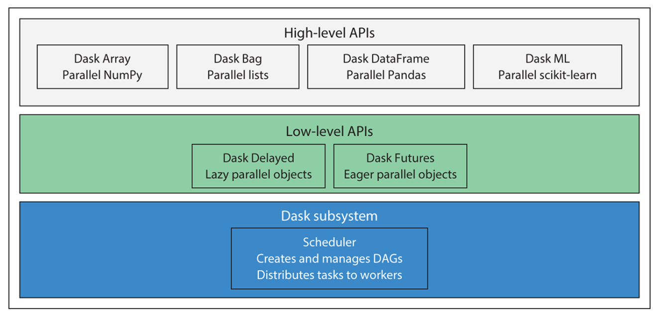
Adapted from Data Science with Python and Dask
1.2 Directed acyclical graph (DAGs)
graph: is a representation of a set of objects that have a relationship with one another >>> good to represent a wide variety of information. A graph is compounded by:
- *node*: a function, an object or an action
- *line*: symbolizes the relationship among nodes
directed acyclical graph: there is one logical way to traverse the graph. No node is visited twice.
cyclical graph: exists a feedback loop that allow to revisit and repeat the actions within the same node.
handle computational resources: as the problem we solve requires more resources we have two options:
-*scale up*: increase size of the available resource. invest in more efficient technology, cons diminishing returns
-*scale out*: add other resources (dask main idea). invest in more cheap resources, cons distribute workload
concurrency: as we approach greater number of "work to be completed", some resources might be not fully exploited. For instance some might be idling because of insufficient shared resources (i.e. resource starvation). Schedulers handle this issue making sure to provide sufficient resources to each worker.
failures:
- work failures: a worker leave, and you know have to assign another one to his task. This might potentially slowing down the execution, however it won't affect previous work (aka data loss)
- data loss: some accident happens and you have to start from the beginning. The scheduler stop and restart from the beginning the whole process.
1.3 Review Part 1
- Dask can be used to scale popular Python libraries such as Pandas and NumPy allowing to analyse dataset with greater size (>8GB)
- Dask uses directed acyclical graph to coordinate execution of parallelized code across processors
- Directed acyclical graph are made up of nodes, clearly defined start and end that can be transverse in only one logical way (no looping).
- Upstream actions are completed before downstream nodes.
- Scaling out (i.e. add workers) can improve performances of complex workloads, however create overhead that can reduces gains.
- In case of failure, the step to reach a node can be repeated from the beginning without disturbing the rest of the process.
Part 2: Introduction to DASK
- Warm up with short example of data cleaning using Dask DataFrames
- Visualize Directed Acyclical Graph generated by Dask workloads with graphviz
- Explore how the scheduler applies the DAGs to coordinate execution code
- You will learn:
- Dask DataFrame API
- Use diagnostic tool
- Use low-level Delayed API to create custom graph
# import libraries
import sys
import os

## import dask libraries
import dask.dataframe as dd
from dask.diagnostics import ProgressBar

# import libraries
import pandas as pd
# assign working directory [CHANGE THIS]. It can not fit in github so I have it locally. Download files
os.chdir('/Users/pavlos/Teaching/2020/AC295_data/nyc-parking-tickets')
cwd = os.getcwd()
# print
print('' , sys.executable)
print('' , cwd)
2.1.2 Load data
## read data using DataFrame API
df = dd.read_csv('Parking_Violations_Issued_-_Fiscal_Year_2017.csv')
df
note that
- metadata are shown in the frame instead of data sample
- syntax is pretty similar to Pandas API
- # partitions is the number of splits used to separate the main dataset. The optimal number is decided by the scheduler that split Pandas DataFrame into smaller chuncks. In this case each partitions is ~64MB (i.e. Dataset size/npartitions = 2GB/33). If we have one worker, Dask will cycle to each partition one at time.
- data types are reported under each column name (similary to describe method in Pandas, however performed through random sampling because data scattered across multiple physical machines). Good practice is to explicit data types instead relying on Dask's inference (store in binary format ideally, see links to Write and Read Parquet).
- Dask Name reports the name of the DAG (i.e. from-delayed)
- # tasks is the number of nodes in the DAG. You can think of a task as a Python function and in this case each partition operates 3 tasks: 1) reading the raw data, 2) splitting the data in appropriate blocks and, 3) initialazing the DataFrame object. Every task comes with some overhead (between 200us and 1ms).
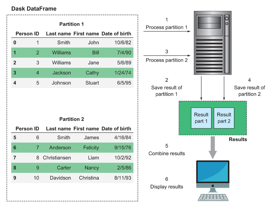
Partition process from Data Science with Python and Dask
Want to know more?
2.1.3 Check data quality issue
# count missing values
missing_values = df.isnull().sum()
missing_values
note that
- dask object created is a series containing metadata and syntax is pretty similar to Pandas API
- processing hasn't be completed yet, instead Dask prepared a DAG stored in the missing values variable (advantage of building graph quickly without need to wait for computation)
- # tasks increased because have been added 2 tasks (i.e. check missing values and sum) for each of the 33 partitions as well as a final addition to aggregate the results among all the partitions for a total of 166 = [(66+1)+99]
# calculate percent missing values
mysize = df.index.size
missing_count = ((missing_values / mysize) * 100)
missing_count
note that
- dask object created is a series and computation hasn't be completed yet
- df.index.size is a dask object dask.dataframe.core.Scalar . You cannot access its value/lenght directely like you would do with a list (e.g. len()). It would go against the whole idea of dask (i.e. read all the dataset)
- # tasks increased because have been added 2 tasks (i.e. division and multiplication)
- data type ahs changed from int64 to float64. Dask automatically converted it once the datatype at the output might not match the input after the division
# run computations using compute method
with ProgressBar():
    missing_count_percent = missing_count.compute()
missing_count_percent
note that
- .compute() method is necessary to run the actions embedded in each node of the DAG
- The results of the compute method are stored into a Pandas Series
- ProgressBar() is a wrapper to keep track of running tasks. It shows completed work
- from a quick visual inspection we can see that are columns that are incomplete and we should drop
2.1.4 Drop columns
# filter sparse columns(greater than 60% missing values) and store them
columns_to_drop = missing_count_percent[missing_count_percent > 60].index
print(columns_to_drop)

# drop sparse columns
with ProgressBar():
    #df_dropped = df.drop(columns_to_drop, axis=1).persist()
    df_dropped = df.drop(columns_to_drop, axis=1).compute()
note that
- use Pandas Series to drop columns in Dask DataFrames because each partition is a Pandas DataFrame
- In the case the Series is made available to all threads, in a cluster it would be serialized and brodcast to all the worker nodes
- .persit() method allows to store in memory intermediate computations so they can be reused.
2.2 Visualize directed acyclic graphs (DAGs)
- DASK uses graphviz library to generate visual representation of the DAGs created by the scheduler
- Use .visualize() metod to inspect the DAGs of DataFrames, Series, Bag, and arrays
- For simplicity we will use Dask Delayed object instead of DataFrames since they grow quite large and hard to visualize
- delayed is a constructor that allows to wrap functions and create Dask Delayed objects that are equivalent to a node in a DAG. By chaining together delayed object, you create the DAG
- Below are two examples, in the first one you build a DAG with one node only with dependencies and in the second one you build another with multiple nodes with dependencies
2.2.1 Example 1: DAG with one node with depenndecy
# import library
import dask.delayed as delayed
def increment(i):
    return i + 1

def add(x, y):
    return x + y

# wrap functions within dealyed object and chain
x = delayed(increment)(1)
y = delayed(increment)(2)
z = delayed(add)(x, y)

# visualize the DAG
z.visualize()

# show the result
z.compute()
note that
- to build a node wrap the function with the delayed object and then pass the arguments of the function. You could also use a decoretors (see documentation).
- circles symbolize function and computations while squares intermediate or final result
- incoming arrows represent dependecies. The increment function do not have any dependency while add function has two. Thus, add function has to wait until objects x and y have been calculated
- functions without dependencies can be computed independentely and a worker can be assigned to each one of them
- use method .visualize() on the last node with dependencies to peak at the DAG
- Dask does not compute the DAG . Use the method .compute() on the last node to see the result
2.2.2 Example 1: DAG with more than one node with dependencies
- we are going to build a more complex DAG with two layers:
- layer1 is built by looping over a list of data using a list comprehension to create dask delayed objects as "leaves" node. This layer combine the previously created function increment with the values in the list, then use the built in function sum to combine the results;
- layer2 is built looping on each object created in layer1 and
data = [1, 2, 3, 4, 5]

# compile first layer and visualize
layer1 = [delayed(increment)(i) for i in data]
total1 = delayed(sum)(layer1)
total1.visualize()

def double(x):
    return x * 2

# compile second layer and visualize
layer2 = [delayed(double)(j) for j in layer1]
total2 = delayed(sum)(layer2)#.persist()
total2.visualize()

z = total2.compute()
z
note that
- built in function
- persistent using .persist() and it will be represented as a rectangle in the graph
## TASK
# visualize DAGs built from the DataFrame
missing_count.visualize()

Want to know more?
2.3 Task scheduling
- Dask performs the so called lazy computations. Remember, until you run the method .compute() all what Dask does is to split the process into smaller logical pieces (which avoid loading all the dataset)
- Even though the process is defined, the number of resources assigned and the place where the results will be stored are note assigned because the scheduler assign them dynamically. This allow to recover from worker failure, network unreliability as well as workers completing the tasks at different speeds.
- Dask uses a central scheduler to orchestrate all this work. It splits the workload among different servers which unlikely they are perfectly assigned the same load, power or access to data. Due to these conditions, scheduler needs to promptly react to avoid bottlenecks that will affect overall runtime.
- For best performance, a Dask cluster should use a distributed file system (S3, HDFS) to back its data storage. Assuming there are two nodes like in the image below and data are stored in one. In order to perform computation in the other node we have to move the data from one to the other creating an overhead proportional to the size of the data. The remedy is to split data minimizing the number of data to broadcast across different local machines.

Local disk from Data Science with Python and Dask
- Dask scheduler takes data locality into consideration when deciding where to perform computation.
2.4 Review Part 2
- The beauty of this code is that you can reuse in one machine or a thousand
- Similar syntax helps transition from Pandas to Dask (good in general for refactoring your code)
- Dask DataFrames is a tool to parallelize computing done popular Pandas that allow to clean and ananlyze large dataset
- Dask parallize Pandas Dataframe and more in general work using DAGs
- Computation are structured by the task scheduler using DAGs
- Computation are constructed lazily and then compute the method
- Use visualize method for a visual representation
- Computation can persist in memory avoid slowdown to replicate result
- Data locality help minimizing network and IO latency
# create lists with actions
action_IDs = [i for i in range(0,10)]
action_description = ['Clean dish', 'Dress up', 'Wash clothes','Take shower','Groceries','Take shower','Dress up','Gym','Take shower','Movie']
action_date = ['2020-1-16', '2020-1-16', '2020-1-16', '2020-1-16', '2020-1-16', '2020-1-17', '2020-1-17', '2020-1-17', '2020-1-17', '2020-1-17']

# store list into Pandas DataFrame
action_pandas_df = pd.DataFrame({'Action ID': action_IDs,
                                 'Action Description': action_description,
                                 'Date': action_date},
                                 columns=['Action ID', 'Action Description', 'Date'])
action_pandas_df
# convert Pandas DataFrame to a Dask DataFrame
action_dask_df = dd.from_pandas(action_pandas_df, npartitions=3)
action_dask_df
# info Dask Dataframe
print('' , action_dask_df.divisions)
print('<# partitions>', action_dask_df.npartitions)
# count rows per partition
action_dask_df.map_partitions(len).compute()
# filter entries in dask dataframe
print('\n ' )
action_filtered = action_dask_df[action_dask_df['Action Description'] != 'Take shower']
print(action_filtered.map_partitions(len).compute())
print('\n ' )
action_filtered_reduced = action_filtered.repartition(npartitions=1)
print(action_filtered_reduced.map_partitions(len).compute())
3.2 Summary part 3 and dask limitations
- dataframe are immutable. Functions such as pop and insert are not supported
- does not allow for functions with a lot of shuffeling like stack/unstack and melt
- limit this operations after major filter and preprocessing
- join, merge, groupby, and rolling are supported but expensive due to shuffeling
- reset index starts sequential counting for each partitions
- apply and iterrow are known to be inefficient in Pandas, the same for Dask
- use .division() to inspect how DataFrame has been partitioned
- for best performance partitions should be rougly equal. Use .repartition() method to balance across datasets
- for best performance sort by logical columns, partition by index and index should be presorted