Key Word(s): Autoencoders, VAE, Variational Autoencoders
 CS109B Data Science 2: Advanced Topics in Data Science
Lab 10 - Autoencoders and Variational Autoencoders
Harvard University
Spring 2019
Instructors: Mark Glickman and Pavlos Protopapas
In [1]:
# !pip install imgaug
In [2]:
## load the libraries
import sys
import warnings
import os
import glob
warnings.filterwarnings("ignore")

import numpy as np
import pandas as pd
import cv2
from sklearn.model_selection import train_test_split

from keras.layers import *
from keras.callbacks import EarlyStopping
from keras.utils import to_categorical
from keras.models import Model, Sequential
from keras.metrics import *
from keras.optimizers import Adam, RMSprop
from scipy.stats import norm
from keras.preprocessing import image

from keras import backend as K

from imgaug import augmenters
import matplotlib.pyplot as plt
plt.gray()
Part 1: Data
Reading data
Download the data given at the following link:
In [3]:
### read dataset
train = pd.read_csv("data/fashion-mnist_train.csv")
train_x = train[list(train.columns)[1:]].values
train_x, val_x = train_test_split(train_x, test_size=0.15)

## create train and validation datasets
train_x, val_x = train_test_split(train_x, test_size=0.15)
In [4]:
## normalize and reshape
train_x = train_x/255.
val_x = val_x/255.

train_x = train_x.reshape(-1, 28, 28, 1)
val_x = val_x.reshape(-1, 28, 28, 1)
In [5]:
train_x.shape
Out[5]:
Visualizing Samples
Visualize 10 images from dataset
In [6]:
f, ax = plt.subplots(1,5)
f.set_size_inches(80, 40)
for i in range(5,10):
    ax[i-5].imshow(train_x[i, :, :, 0].reshape(28, 28))

Part 2: Denoise Images using AEs
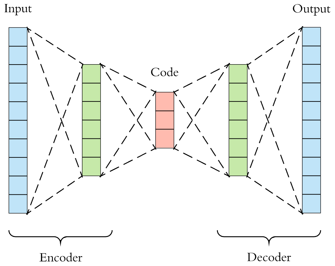
Understanding AEs
Add Noise to Images
Check out imgaug docs for more info and other ways to add noise.
In [7]:
# Lets add sample noise - Salt and Pepper
noise = augmenters.SaltAndPepper(0.1)
seq_object = augmenters.Sequential([noise])

train_x_n = seq_object.augment_images(train_x * 255) / 255
val_x_n = seq_object.augment_images(val_x * 255) / 255
In [8]:
f, ax = plt.subplots(1,5)
f.set_size_inches(80, 40)
for i in range(5,10):
    ax[i-5].imshow(train_x_n[i, :, :, 0].reshape(28, 28))

Setup Encoder Neural Network
Try different number of hidden layers, nodes?
In [9]:
# input layer
input_layer = Input(shape=(28, 28, 1))

# encoding architecture
encoded_layer1 = Conv2D(64, (3, 3), activation='relu', padding='same')(input_layer)
encoded_layer1 = MaxPool2D( (2, 2), padding='same')(encoded_layer1)
encoded_layer2 = Conv2D(32, (3, 3), activation='relu', padding='same')(encoded_layer1)
encoded_layer2 = MaxPool2D( (2, 2), padding='same')(encoded_layer2)
encoded_layer3 = Conv2D(16, (3, 3), activation='relu', padding='same')(encoded_layer2)
latent_view    = MaxPool2D( (2, 2), padding='same')(encoded_layer3)
Setup Decoder Neural Network
Try different number of hidden layers, nodes?
In [10]:
# decoding architecture
decoded_layer1 = Conv2D(16, (3, 3), activation='relu', padding='same')(latent_view)
decoded_layer1 = UpSampling2D((2, 2))(decoded_layer1)
decoded_layer2 = Conv2D(32, (3, 3), activation='relu', padding='same')(decoded_layer1)
decoded_layer2 = UpSampling2D((2, 2))(decoded_layer2)
decoded_layer3 = Conv2D(64, (3, 3), activation='relu')(decoded_layer2)
decoded_layer3 = UpSampling2D((2, 2))(decoded_layer3)
output_layer   = Conv2D(1, (3, 3), padding='same')(decoded_layer3)
Train AE
In [11]:
# compile the model
model = Model(input_layer, output_layer)
model.compile(optimizer='adam', loss='mse')
In [12]:
model.summary()
In [13]:
early_stopping = EarlyStopping(monitor='val_loss', min_delta=0, patience=10, verbose=5, mode='auto')
history = model.fit(train_x_n, train_x, epochs=20, batch_size=2048, validation_data=(val_x_n, val_x), callbacks=[early_stopping])
Visualize Intermediate Layers of AE
Visualize intermediate layers
In [14]:
# compile the model
model_2 = Model(input_layer, latent_view)
model_2.compile(optimizer='adam', loss='mse')
In [15]:
n = np.random.randint(0,len(val_x)-5)
f, ax = plt.subplots(1,5)
f.set_size_inches(80, 40)
for i,a in enumerate(range(n,n+5)):
    ax[i].imshow(val_x_n[a, :, :, 0].reshape(28, 28))
plt.show()

In [16]:
preds = model_2.predict(val_x_n[n:n+5])
preds.shape
Out[16]:
In [17]:
f, ax = plt.subplots(16,5)
ax = ax.ravel()
f.set_size_inches(20, 40)
for j in range(16):
    for i,a in enumerate(range(n,n+5)):
        ax[j*5 + i].imshow(preds[i, :, :, j])
plt.show()

Visualize Samples reconstructed by AE
In [18]:
n = np.random.randint(0,len(val_x)-5)
In [19]:
f, ax = plt.subplots(1,5)
f.set_size_inches(80, 40)
for i,a in enumerate(range(n,n+5)):
    ax[i].imshow(val_x[a, :, :, 0].reshape(28, 28))

In [20]:
f, ax = plt.subplots(1,5)
f.set_size_inches(80, 40)
for i,a in enumerate(range(n,n+5)):
    ax[i].imshow(val_x_n[a, :, :, 0].reshape(28, 28))

In [21]:
preds = model.predict(val_x_n[n:n+5])
f, ax = plt.subplots(1,5)
f.set_size_inches(80, 40)
for i,a in enumerate(range(n,n+5)):
    ax[i].imshow(preds[i].reshape(28, 28))
plt.show()

Part 3: Exercise: Denoising noisy documents
In [22]:
TRAIN_IMAGES = glob.glob('data/train/*.png')
CLEAN_IMAGES = glob.glob('data/train_cleaned/*.png')
TEST_IMAGES = glob.glob('data/test/*.png')
In [23]:
plt.figure(figsize=(20,8))
img = cv2.imread('data/train/101.png', 0)
plt.imshow(img, cmap='gray')
print(img.shape)

In [24]:
def load_image(path):
    image_list = np.zeros((len(path), 258, 540, 1))
    for i, fig in enumerate(path):
        img = image.load_img(fig, grayscale=True, target_size=(258, 540))
        x = image.img_to_array(img).astype('float32')
        x = x / 255.0
        image_list[i] = x

    return image_list

x_train = load_image(TRAIN_IMAGES)
y_train = load_image(CLEAN_IMAGES)
x_test = load_image(TEST_IMAGES)

print(x_train.shape, x_test.shape)
In [1]:
#Todo: Split your dataset into train and val
In [2]:
#Todo: Visualize your train set
In [3]:
input_layer = Input(shape=(258, 540, 1))

#Todo: Setup encoder
#Hint: Conv2D - > MaxPooling

#Todo: Setup decoder
#Hint: Conv2D - > Upsampling

output_layer = Conv2D(1, (3, 3), activation='sigmoid', padding='same')(decoder)

ae = Model(input_layer, output_layer)
In [4]:
#Todo: Compile and summarize your auto encoder
In [5]:
#Todo: Train your autoencoder
In [32]:
preds = ae.predict(x_test)
In [6]:
# n = 25
# preds_0 = preds[n] * 255.0
# preds_0 = preds_0.reshape(258, 540)
# x_test_0 = x_test[n] * 255.0
# x_test_0 = x_test_0.reshape(258, 540)
# plt.imshow(x_test_0, cmap='gray')
In [7]:
# plt.imshow(preds_0, cmap='gray')
Part 4: Generating New Fashion using VAEs
Understanding VAEs

Reset data
In [35]:
### read dataset
train = pd.read_csv("data/fashion-mnist_train.csv")
train_x = train[list(train.columns)[1:]].values
train_x, val_x = train_test_split(train_x, test_size=0.2)

## create train and validation datasets
train_x, val_x = train_test_split(train_x, test_size=0.2)
In [36]:
## normalize and reshape
train_x = train_x/255.
val_x = val_x/255.

train_x = train_x.reshape(-1, 28, 28, 1)
val_x = val_x.reshape(-1, 28, 28, 1)
Setup Encoder Neural Network
Try different number of hidden layers, nodes?
In [37]:
import keras.backend as K
In [38]:
batch_size = 16
latent_dim = 2  # Number of latent dimension parameters

input_img = Input(shape=(784,), name="input")
x = Dense(512, activation='relu', name="intermediate_encoder")(input_img)
x = Dense(2, activation='relu', name="latent_encoder")(x)

z_mu = Dense(latent_dim)(x)
z_log_sigma = Dense(latent_dim)(x)
In [39]:
# sampling function
def sampling(args):
    z_mu, z_log_sigma = args
    epsilon = K.random_normal(shape=(K.shape(z_mu)[0], latent_dim),
                              mean=0., stddev=1.)
    return z_mu + K.exp(z_log_sigma) * epsilon

# sample vector from the latent distribution
z = Lambda(sampling)([z_mu, z_log_sigma])
In [40]:
# decoder takes the latent distribution sample as input
decoder_input = Input((2,), name="input_decoder")

x = Dense(512, activation='relu', name="intermediate_decoder", input_shape=(2,))(decoder_input)

# Expand to 784 total pixels
x = Dense(784, activation='sigmoid', name="original_decoder")(x)

# decoder model statement
decoder = Model(decoder_input, x)

# apply the decoder to the sample from the latent distribution
z_decoded = decoder(z)
In [41]:
decoder.summary()
In [42]:
# construct a custom layer to calculate the loss
class CustomVariationalLayer(Layer):

    def vae_loss(self, x, z_decoded):
        x = K.flatten(x)
        z_decoded = K.flatten(z_decoded)
        # Reconstruction loss
        xent_loss = binary_crossentropy(x, z_decoded)
        return xent_loss

    # adds the custom loss to the class
    def call(self, inputs):
        x = inputs[0]
        z_decoded = inputs[1]
        loss = self.vae_loss(x, z_decoded)
        self.add_loss(loss, inputs=inputs)
        return x

# apply the custom loss to the input images and the decoded latent distribution sample
y = CustomVariationalLayer()([input_img, z_decoded])
In [43]:
z_decoded
Out[43]:
In [44]:
# VAE model statement
vae = Model(input_img, y)
vae.compile(optimizer='rmsprop', loss=None)
In [45]:
vae.summary()
In [46]:
train_x.shape
Out[46]:
In [47]:
train_x = train_x.reshape(-1, 784)
val_x = val_x.reshape(-1, 784)
In [48]:
vae.fit(x=train_x, y=None,
        shuffle=True,
        epochs=20,
        batch_size=batch_size,
        validation_data=(val_x, None))
Out[48]:
In [49]:
# Display a 2D manifold of the samples
n = 20  # figure with 20x20 samples
digit_size = 28
figure = np.zeros((digit_size * n, digit_size * n))

# Construct grid of latent variable values - can change values here to generate different things
grid_x = norm.ppf(np.linspace(0.05, 0.95, n))
grid_y = norm.ppf(np.linspace(0.05, 0.95, n))

# decode for each square in the grid
for i, yi in enumerate(grid_x):
    for j, xi in enumerate(grid_y):
        z_sample = np.array([[xi, yi]])
        z_sample = np.tile(z_sample, batch_size).reshape(batch_size, 2)

        x_decoded = decoder.predict(z_sample, batch_size=batch_size)

        digit = x_decoded[0].reshape(digit_size, digit_size)

        figure[i * digit_size: (i + 1) * digit_size,
               j * digit_size: (j + 1) * digit_size] = digit

plt.figure(figsize=(20, 20))
plt.imshow(figure)
plt.show()

In [50]:
### read dataset
train = pd.read_csv("fashion-mnist_train.csv")
train_x = train[list(train.columns)[1:]].values
train_y = train[list(train.columns)[0]].values

train_x = train_x/255.
# train_x = train_x.reshape(-1, 28, 28, 1)

# Translate into the latent space
encoder = Model(input_img, z_mu)
x_valid_noTest_encoded = encoder.predict(train_x, batch_size=batch_size)
plt.figure(figsize=(10, 10))
plt.scatter(x_valid_noTest_encoded[:, 0], x_valid_noTest_encoded[:, 1], c=train_y, cmap='brg')
plt.colorbar()
plt.show()

Part 5: Exercise: Generating New Fashion using VAEs: Adding CNNs and KL Divergence Loss
In [8]:
batch_size = 16
latent_dim = 2  # Number of latent dimension parameters

# Hint: Encoder architecture: Input -> Conv2D*4 -> Flatten -> Dense
input_img = Input(shape=(28, 28, 1))


#Todo: Setup encoder network

shape_before_flattening = K.int_shape(x)

x = Flatten()(x)
x = Dense(32, activation='relu')(x)

# Two outputs, latent mean and (log)variance
z_mu = Dense(latent_dim)(x)
z_log_sigma = Dense(latent_dim)(x)
Set up sampling function
In [52]:
# sampling function
def sampling(args):
    z_mu, z_log_sigma = args
    epsilon = K.random_normal(shape=(K.shape(z_mu)[0], latent_dim),
                              mean=0., stddev=1.)
    return z_mu + K.exp(z_log_sigma) * epsilon

# sample vector from the latent distribution
z = Lambda(sampling)([z_mu, z_log_sigma])
Setup Decoder Neural Network
Try different number of hidden layers, nodes?
In [9]:
# decoder takes the latent distribution sample as input
decoder_input = Input(K.int_shape(z)[1:])

#Todo: Setup decoder network
#Hint Expand to 784 pixels -> reshape -> Conv2Dtranspose -> conv2D

# decoder model statement
decoder = Model(decoder_input, x)

# apply the decoder to the sample from the latent distribution
z_decoded = decoder(z)
Set up loss functions
In [54]:
# construct a custom layer to calculate the loss
class CustomVariationalLayer(Layer):

    def vae_loss(self, x, z_decoded):
        x = K.flatten(x)
        z_decoded = K.flatten(z_decoded)
        # Reconstruction loss
        xent_loss = binary_crossentropy(x, z_decoded)
        # KL divergence
        kl_loss = -5e-4 * K.mean(1 + z_log_sigma - K.square(z_mu) - K.exp(z_log_sigma), axis=-1)
        return K.mean(xent_loss + kl_loss)

    # adds the custom loss to the class
    def call(self, inputs):
        x = inputs[0]
        z_decoded = inputs[1]
        loss = self.vae_loss(x, z_decoded)
        self.add_loss(loss, inputs=inputs)
        return x

# apply the custom loss to the input images and the decoded latent distribution sample
y = CustomVariationalLayer()([input_img, z_decoded])
Train VAE
In [55]:
# VAE model statement
vae = Model(input_img, y)
vae.compile(optimizer='rmsprop', loss=None)
In [10]:
vae.summary()
In [57]:
train_x = train_x.reshape(-1, 28, 28, 1)
val_x = val_x.reshape(-1, 28, 28, 1)
In [11]:
vae.fit(x=train_x, y=None,
        shuffle=True,
        epochs=20,
        batch_size=batch_size,
        validation_data=(val_x, None))
Visualize Samples reconstructed by VAE
In [12]:
# Display a 2D manifold of the samples
n = 20  # figure with 20x20 samples
digit_size = 28
figure = np.zeros((digit_size * n, digit_size * n))

# Construct grid of latent variable values - can change values here to generate different things
grid_x = norm.ppf(np.linspace(0.05, 0.95, n))
grid_y = norm.ppf(np.linspace(0.05, 0.95, n))

# decode for each square in the grid
for i, yi in enumerate(grid_x):
    for j, xi in enumerate(grid_y):
        z_sample = np.array([[xi, yi]])
        z_sample = np.tile(z_sample, batch_size).reshape(batch_size, 2)
        x_decoded = decoder.predict(z_sample, batch_size=batch_size)
        digit = x_decoded[0].reshape(digit_size, digit_size)
        figure[i * digit_size: (i + 1) * digit_size,
               j * digit_size: (j + 1) * digit_size] = digit

plt.figure(figsize=(20, 20))
plt.imshow(figure)
plt.show()
Exercise: Visualize latent space
In [60]:
train = pd.read_csv("data/fashion-mnist_train.csv")
In [61]:
### read dataset
train = pd.read_csv("data/fashion-mnist_train.csv")
train_x = train[list(train.columns)[1:]].values
train_y = train[list(train.columns)[0]].values

train_x = train_x/255.
train_x = train_x.reshape(-1, 28, 28, 1)
In [13]:
# Translate into the latent space
encoder = Model(input_img, z_mu)
x_valid_noTest_encoded = encoder.predict(train_x, batch_size=batch_size)
plt.figure(figsize=(10, 10))
plt.scatter(x_valid_noTest_encoded[:, 0], x_valid_noTest_encoded[:, 1], c=train_y, cmap='brg')
plt.colorbar()
plt.show()