Key Word(s): Matplotlib, Simple Linear Regression, kNN, array reshape, sklearn, statsmodels
 CS109A Introduction to Data Science
Lab 3: plotting, K-NN Regression, Simple Linear Regression
Harvard University
Fall 2019
Instructors: Pavlos Protopapas, Kevin Rader, and Chris Tanner
Material prepared by: David Sondak, Will Claybaugh, Pavlos Protopapas, and Eleni Kaxiras.
#RUN THIS CELL
import requests
from IPython.core.display import HTML
styles = requests.get("https://raw.githubusercontent.com/Harvard-IACS/2018-CS109A/master/content/styles/cs109.css").text
HTML(styles)
Learning Goals
By the end of this lab, you should be able to:
- Review
numpyincluding 2-D arrays and understand array reshaping - Use
matplotlibto make plots - Feel comfortable with simple linear regression
- Feel comfortable with $k$ nearest neighbors
This lab corresponds to lectures 4 and 5 and maps on to homework 2 and beyond.
import numpy as np
import scipy as sp
import matplotlib as mpl
import matplotlib.cm as cm
import matplotlib.pyplot as plt
import pandas as pd
import time
pd.set_option('display.width', 500)
pd.set_option('display.max_columns', 100)
pd.set_option('display.notebook_repr_html', True)
#import seaborn as sns
import warnings
warnings.filterwarnings('ignore')
# Displays the plots for us.
%matplotlib inline
# Use this as a variable to load solutions: %load PATHTOSOLUTIONS/exercise1.py. It will be substituted in the code
# so do not worry if it disappears after you run the cell.
PATHTOSOLUTIONS = 'solutions'
1 - Review of the numpy Python library
In lab1 we learned about the numpy library (documentation) and its fast array structure, called the numpy array.
# import numpy
import numpy as np
# make an array
my_array = np.array([1,4,9,16])
my_array
print(f'Size of my array: {my_array.size}, or length of my array: {len(my_array)}')
print (f'Shape of my array: {my_array.shape}')
Notice the way the shape appears in numpy arrays
- For a 1D array, .shape returns a tuple with 1 element (n,)
- For a 2D array, .shape returns a tuple with 2 elements (n,m)
- For a 3D array, .shape returns a tuple with 3 elements (n,m,p)
# How to reshape a 1D array to a 2D
my_array.reshape(-1,2)
Numpy arrays support the same operations as lists! Below we slice and iterate.
print("array[2:4]:", my_array[2:4]) # A slice of the array

# Iterate over the array
for ele in my_array:
    print("element:", ele)
Remember numpy gains a lot of its efficiency from being strongly typed (all elements are of the same type, such as integer or floating point). If the elements of an array are of a different type, numpy will force them into the same type (the longest in terms of bytes)
mixed = np.array([1, 2.3, 'eleni', True])
print(type(1), type(2.3), type('eleni'), type(True))
mixed # all elements will become strings
Next, we push ahead to two-dimensional arrays and begin to dive into some of the deeper aspects of numpy.
# create a 2d-array by handing a list of lists
my_array2d = np.array([ [1, 2, 3, 4],
                        [5, 6, 7, 8],
                        [9, 10, 11, 12]
])

my_array2d
Array Slicing (a reminder...)
Numpy arrays can be sliced, and can be iterated over with loops. Below is a schematic illustrating slicing two-dimensional arrays.
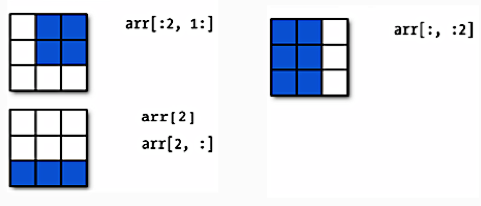
Notice that the list slicing syntax still works!
array[2:,3] says "in the array, get rows 2 through the end, column 3]"
array[3,:] says "in the array, get row 3, all columns".
Pandas Slicing (a reminder...)
.iloc is by position (position is unique), .loc is by label (label is not unique)
# import cast dataframe
cast = pd.read_csv('../data/cast.csv', encoding='utf_8')
cast.head()
# get me rows 10 to 13 (python slicing style : exclusive of end)
cast.iloc[10:13]
# get me columns 0 to 2 but all rows - use head()
cast.iloc[:, 0:2].head()
# get me rows 10 to 13 AND only columns 0 to 2
cast.iloc[10:13, 0:2]
# COMPARE: get me rows 10 to 13 (pandas slicing style : inclusive of end)
cast.loc[10:13]
# give me columns 'year' and 'type' by label but only for rows 5 to 10
cast.loc[5:10,['year','type']]
Python Trick of the Day
import re
names = ['mayday','springday','horseday','june']
# TODO : substitute these lines code with 1 line of code using list comprehension

cleaned = []
for name in names:
    this = re.sub('[Dd]ay$', '', name)
    cleaned.append(this)
cleaned
# your code here
# solution
cleaned2 = [re.sub('[Dd]ay$', '', name) for name in names]
cleaned2
2 - Plotting with matplotlib and beyond
matplotlib is a very powerful python library for making scientific plots.
We will not focus too much on the internal aspects of matplotlib in today's lab. There are many excellent tutorials out there for matplotlib. For example,
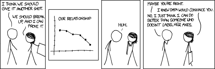
Conveying your findings convincingly is an absolutely crucial part of any analysis. Therefore, you must be able to write well and make compelling visuals. Creating informative visuals is an involved process and we won't cover that in this lab. However, part of creating informative data visualizations means generating readable figures. If people can't read your figures or have a difficult time interpreting them, they won't understand the results of your work. Here are some non-negotiable commandments for any plot:
- Label $x$ and $y$ axes
- Axes labels should be informative
- Axes labels should be large enough to read
- Make tick labels large enough
- Include a legend if necessary
- Include a title if necessary
- Use appropriate line widths
- Use different line styles for different lines on the plot
- Use different markers for different lines
There are other important elements, but that list should get you started on your way.
We will work with matplotlib and seaborn for plotting in this class. matplotlib is a very powerful python library for making scientific plots. seaborn is a little more specialized in that it was developed for statistical data visualization. We will cover some seaborn later in class. In the meantime you can look at the seaborn documentation
First, let's generate some data.
Let's plot some functions
We will use the following three functions to make some plots:
- Logistic function: \begin{align*} f\left(z\right) = \dfrac{1}{1 + be^{-az}} \end{align*} where $a$ and $b$ are parameters.
- Hyperbolic tangent: \begin{align*} g\left(z\right) = b\tanh\left(az\right) + c \end{align*} where $a$, $b$, and $c$ are parameters.
- Rectified Linear Unit:
\begin{align*}
h\left(z\right) =
\left{
\right. \end{align*} where $\epsilon < 0$ is a small, positive parameter.\begin{array}{lr} z, \quad z > 0 \\ \epsilon z, \quad z\leq 0 \end{array}
You are given the code for the first two functions. Notice that $z$ is passed in as a numpy array and that the functions are returned as numpy arrays. Parameters are passed in as floats.
You should write a function to compute the rectified linear unit. The input should be a numpy array for $z$ and a positive float for $\epsilon$.
import numpy as np

def logistic(z: np.ndarray, a: float, b: float) -> np.ndarray:
    """ Compute logistic function
      Inputs:
         a: exponential parameter
         b: exponential prefactor
         z: numpy array; domain
      Outputs:
         f: numpy array of floats, logistic function
    """

    den = 1.0 + b * np.exp(-a * z)
    return 1.0 / den

def stretch_tanh(z: np.ndarray, a: float, b: float, c: float) -> np.ndarray:
    """ Compute stretched hyperbolic tangent
      Inputs:
         a: horizontal stretch parameter (a>1 implies a horizontal squish)
         b: vertical stretch parameter
         c: vertical shift parameter
         z: numpy array; domain
      Outputs:
         g: numpy array of floats, stretched tanh
    """
    return b * np.tanh(a * z) + c

def relu(z: np.ndarray, eps: float = 0.01) -> np.ndarray:
    """ Compute rectificed linear unit
      Inputs:
         eps: small positive parameter
         z: numpy array; domain
      Outputs:
         h: numpy array; relu
    """
    return np.fmax(z, eps * z)
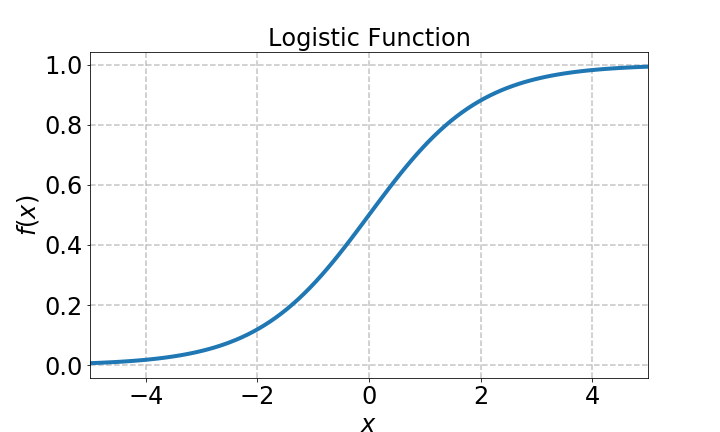
Now let's make some plots. First, let's just warm up and plot the logistic function.
x = np.linspace(-5.0, 5.0, 100) # Equally spaced grid of 100 pts between -5 and 5

f = logistic(x, 1.0, 1.0) # Generate data
plt.plot(x, f)
plt.xlabel('x')
plt.ylabel('f')
plt.title('Logistic Function')
plt.grid(True)

Figures with subplots
Let's start thinking about the plots as objects. We have the figure object which is like a matrix of smaller plots named axes. You can use array notation when handling it.
fig, ax = plt.subplots(1,1) # Get figure and axes objects

ax.plot(x, f) # Make a plot

# Create some labels
ax.set_xlabel('x')
ax.set_ylabel('f')
ax.set_title('Logistic Function')

# Grid
ax.grid(True)
Wow, it's exactly the same plot! Notice, however, the use of ax.set_xlabel() instead of plt.xlabel(). The difference is tiny, but you should be aware of it. I will use this plotting syntax from now on.
What else do we need to do to make this figure better? Here are some options:
- Make labels bigger!
- Make line fatter
- Make tick mark labels bigger
- Make the grid less pronounced
- Make figure bigger
Let's get to it.
fig, ax = plt.subplots(1,1, figsize=(10,6)) # Make figure bigger

# Make line plot
ax.plot(x, f, lw=4)

# Update ticklabel size
ax.tick_params(labelsize=24)

# Make labels
ax.set_xlabel(r'$x$', fontsize=24) # Use TeX for mathematical rendering
ax.set_ylabel(r'$f(x)$', fontsize=24) # Use TeX for mathematical rendering
ax.set_title('Logistic Function', fontsize=24)

ax.grid(True, lw=1.5, ls='--', alpha=0.75)

Notice:
lwstands forlinewidth. We could also writeax.plot(x, f, linewidth=4)lsstands forlinestyle.alphastands for transparency.
The only thing remaining to do is to change the $x$ limits. Clearly these should go from $-5$ to $5$.
#fig.savefig('logistic.png')
# Put this in a markdown cell and uncomment this to check what you saved.
# 
Resources
If you want to see all the styles available, please take a look at the documentation.
We haven't discussed it yet, but you can also put a legend on a figure. You'll do that in the next exercise. Here are some additional resources:
ax.legend(loc='best', fontsize=24);
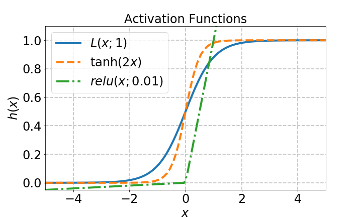
Do the following:
- Make a figure with the logistic function, hyperbolic tangent, and rectified linear unit.
- Use different line styles for each plot
- Put a legend on your figure
Here's an example of a figure:
# your code here

# First get the data
f = logistic(x, 2.0, 1.0)
g = stretch_tanh(x, 2.0, 0.5, 0.5)
h = relu(x)

fig, ax = plt.subplots(1,1, figsize=(10,6)) # Create figure object

# Make actual plots
# (Notice the label argument!)
ax.plot(x, f, lw=4, ls='-', label=r'$L(x;1)$')
ax.plot(x, g, lw=4, ls='--', label=r'$\tanh(2x)$')
ax.plot(x, h, lw=4, ls='-.', label=r'$relu(x; 0.01)$')

# Make the tick labels readable
ax.tick_params(labelsize=24)

# Set axes limits to make the scale nice
ax.set_xlim(x.min(), x.max())
ax.set_ylim(h.min(), 1.1)

# Make readable labels
ax.set_xlabel(r'$x$', fontsize=24)
ax.set_ylabel(r'$h(x)$', fontsize=24)
ax.set_title('Activation Functions', fontsize=24)

# Set up grid
ax.grid(True, lw=1.75, ls='--', alpha=0.75)

# Put legend on figure
ax.legend(loc='best', fontsize=24);

fig.savefig('../images/nice_plots.png')

These figures look nice in the plot and it makes sense for comparison. Now let's put the 3 different figures in separate plots.
- Make a separate plot for each figure and line them up on the same row.
# your code here
# %load solutions/three_subplots.py
# First get the data
f = logistic(x, 2.0, 1.0)
g = stretch_tanh(x, 2.0, 0.5, 0.5)
h = relu(x)

fig, ax = plt.subplots(1,3, figsize=(20,6)) # Create figure object

# Make actual plots
ax[0].plot(x, f, lw=4, ls='-', label=r'$L(x;1)$')
ax[1].plot(x, g, lw=4, ls='--', label=r'$\tanh(2x)$')
ax[2].plot(x, h, lw=4, ls='-.', label=r'$relu(x; 0.01)$')

# Make the tick labels readable
ax[0].tick_params(labelsize=24)
ax[1].tick_params(labelsize=24)
ax[2].tick_params(labelsize=24)

# Set axes limits to make the scale nice
ax[0].set_xlim(x.min(), x.max())
ax[0].set_ylim(h.min(), 1.1)
ax[1].set_xlim(x.min(), x.max())
ax[1].set_ylim(h.min(), 1.1)
ax[2].set_xlim(x.min(), x.max())
ax[2].set_ylim(h.min(), 1.1)

# Make readable labels
ax[0].set_xlabel(r'$x$', fontsize=24)
ax[0].set_ylabel(r'$h(x)$', fontsize=24)
ax[0].set_title('Activation Functions', fontsize=24)

ax[1].set_xlabel(r'$x$', fontsize=24)
ax[1].set_ylabel(r'$h(x)$', fontsize=24)
ax[1].set_title('Activation Functions', fontsize=24)

ax[2].set_xlabel(r'$x$', fontsize=24)
ax[2].set_ylabel(r'$h(x)$', fontsize=24)
ax[2].set_title('Activation Functions', fontsize=24)

# Set up grid
ax[0].grid(True, lw=1.75, ls='--', alpha=0.75)
ax[1].grid(True, lw=1.75, ls='--', alpha=0.75)
ax[2].grid(True, lw=1.75, ls='--', alpha=0.75)

# Put legend on figure
ax[0].legend(loc='best', fontsize=24);
ax[1].legend(loc='best', fontsize=24);
ax[2].legend(loc='best', fontsize=24);

#fig.savefig('../images/nice_sub_plots.png')

- Make a grid of 2 x 3 separate plots, 3 will be empty. Just plot the functions and do not worry about cosmetics. We just want you ro see the functionality.
# your code here
# %load solutions/six_subplots.py

# First get the data
f = logistic(x, 2.0, 1.0)
g = stretch_tanh(x, 2.0, 0.5, 0.5)
h = relu(x)

fig, ax = plt.subplots(2,3, figsize=(20,6)) # Create figure object

# Make actual plots
ax[0][0].plot(x, f, lw=4, ls='-', label=r'$L(x;1)$')
ax[1][1].plot(x, g, lw=4, ls='--', label=r'$\tanh(2x)$')
ax[1][2].plot(x, h, lw=4, ls='-.', label=r'$relu(x; 0.01)$')
ax[0][2].plot(x, h, lw=4, ls='-.', label=r'$relu(x; 0.01)$')

3 - Simple Linear Regression
Linear regression and its many extensions are a workhorse of the statistics and data science community, both in application and as a reference point for other models. Most of the major concepts in machine learning can be and often are discussed in terms of various linear regression models. Thus, this section will introduce you to building and fitting linear regression models and some of the process behind it, so that you can 1) fit models to data you encounter 2) experiment with different kinds of linear regression and observe their effects 3) see some of the technology that makes regression models work.
Linear regression with a toy dataset
We first examine a toy problem, focusing our efforts on fitting a linear model to a small dataset with three observations. Each observation consists of one predictor $x_i$ and one response $y_i$ for $i = 1, 2, 3$,
\begin{align*} (x , y) = \{(x_1, y_1), (x_2, y_2), (x_3, y_3)\}. \end{align*}To be very concrete, let's set the values of the predictors and responses.
\begin{equation*} (x , y) = \{(1, 2), (2, 2), (3, 4)\} \end{equation*}There is no line of the form $\beta_0 + \beta_1 x = y$ that passes through all three observations, since the data are not collinear. Thus our aim is to find the line that best fits these observations in the least-squares sense, as discussed in lecture.
- Make two numpy arrays out of this data, x_train and y_train
- Check the dimentions of these arrays
- Try to reshape them into a different shape
- Make points into a very simple scatterplot
- Make a better scatterplot
# your code here
# solution
x_train = np.array([1,2,3])
y_train = np.array([2,3,6])
type(x_train)
x_train.shape
x_train = x_train.reshape(3,1)
x_train.shape
# %load solutions/simple_scatterplot.py
# Make a simple scatterplot
plt.scatter(x_train,y_train)

# check dimensions
print(x_train.shape,y_train.shape)

# %load solutions/nice_scatterplot.py
def nice_scatterplot(x, y, title):
    # font size
    f_size = 18

    # make the figure
    fig, ax = plt.subplots(1,1, figsize=(8,5)) # Create figure object

    # set axes limits to make the scale nice
    ax.set_xlim(np.min(x)-1, np.max(x) + 1)
    ax.set_ylim(np.min(y)-1, np.max(y) + 1)

    # adjust size of tickmarks in axes
    ax.tick_params(labelsize = f_size)

    # remove tick labels
    ax.tick_params(labelbottom=False,  bottom=False)

    # adjust size of axis label
    ax.set_xlabel(r'$x$', fontsize = f_size)
    ax.set_ylabel(r'$y$', fontsize = f_size)

    # set figure title label
    ax.set_title(title, fontsize = f_size)

    # you may set up grid with this
    ax.grid(True, lw=1.75, ls='--', alpha=0.15)

    # make actual plot (Notice the label argument!)
    #ax.scatter(x, y, label=r'$my points$')
    #ax.scatter(x, y, label='$my points$')
    ax.scatter(x, y, label=r'$my\,points$')
    ax.legend(loc='best', fontsize = f_size);

    return ax

nice_scatterplot(x_train, y_train, 'hello nice plot')

Formulae
Linear regression is special among the models we study because it can be solved explicitly. While most other models (and even some advanced versions of linear regression) must be solved itteratively, linear regression has a formula where you can simply plug in the data.
For the single predictor case it is: \begin{align} \beta_1 &= \frac{\sum_{i=1}^n{(x_i-\bar{x})(y_i-\bar{y})}}{\sum_{i=1}^n{(x_i-\bar{x})^2}}\\ \beta_0 &= \bar{y} - \beta_1\bar{x}\ \end{align}
Where $\bar{y}$ and $\bar{x}$ are the mean of the y values and the mean of the x values, respectively.
Building a model from scratch
In this part, we will solve the equations for simple linear regression and find the best fit solution to our toy problem.
The snippets of code below implement the linear regression equations on the observed predictors and responses, which we'll call the training data set. Let's walk through the code.
We have to reshape our arrrays to 2D. We will see later why.
- make an array with shape (2,3)
- reshape it to a size that you want
# your code here
#solution
xx = np.array([[1,2,3],[4,6,8]])
xxx = xx.reshape(-1,2)
xxx.shape
# Reshape to be a proper 2D array
x_train = x_train.reshape(x_train.shape[0], 1)
y_train = y_train.reshape(y_train.shape[0], 1)

print(x_train.shape)
# first, compute means
y_bar = np.mean(y_train)
x_bar = np.mean(x_train)

# build the two terms
numerator = np.sum( (x_train - x_bar)*(y_train - y_bar) )
denominator = np.sum((x_train - x_bar)**2)

print(numerator.shape, denominator.shape) #check shapes
- Why the empty brackets? (The numerator and denominator are scalars, as expected.)
#slope beta1
beta_1 = numerator/denominator

#intercept beta0
beta_0 = y_bar - beta_1*x_bar

print("The best-fit line is {0:3.2f} + {1:3.2f} * x".format(beta_0, beta_1))
print(f'The best fit is {beta_0}')
Turn the code from the above cells into a function called simple_linear_regression_fit, that inputs the training data and returns beta0 and beta1.
To do this, copy and paste the code from the above cells below and adjust the code as needed, so that the training data becomes the input and the betas become the output.
def simple_linear_regression_fit(x_train: np.ndarray, y_train: np.ndarray) -> np.ndarray:

    return
Check your function by calling it with the training data from above and printing out the beta values.
# Your code here
# %load solutions/simple_linear_regression_fit.py
def simple_linear_regression_fit(x_train: np.ndarray, y_train: np.ndarray) -> np.ndarray:
    """
    Inputs:
    x_train: a (num observations by 1) array holding the values of the predictor variable
    y_train: a (num observations by 1) array holding the values of the response variable

    Returns:
    beta_vals:  a (num_features by 1) array holding the intercept and slope coeficients
    """

    # Check input array sizes
    if len(x_train.shape) < 2:
        print("Reshaping features array.")
        x_train = x_train.reshape(x_train.shape[0], 1)

    if len(y_train.shape) < 2:
        print("Reshaping observations array.")
        y_train = y_train.reshape(y_train.shape[0], 1)

    # first, compute means
    y_bar = np.mean(y_train)
    x_bar = np.mean(x_train)

    # build the two terms
    numerator = np.sum( (x_train - x_bar)*(y_train - y_bar) )
    denominator = np.sum((x_train - x_bar)**2)

    #slope beta1
    beta_1 = numerator/denominator

    #intercept beta0
    beta_0 = y_bar - beta_1*x_bar

    return np.array([beta_0,beta_1])
- Let's run this function and see the coefficients
x_train = np.array([1 ,2, 3])
y_train = np.array([2, 2, 4])

betas = simple_linear_regression_fit(x_train, y_train)

beta_0 = betas[0]
beta_1 = betas[1]

print("The best-fit line is {0:8.6f} + {1:8.6f} * x".format(beta_0, beta_1))
- Do the values of
beta0andbeta1seem reasonable? - Plot the training data using a scatter plot.
- Plot the best fit line with
beta0andbeta1together with the training data.
# Your code here
# %load solutions/best_fit_scatterplot.py
fig_scat, ax_scat = plt.subplots(1,1, figsize=(10,6))

# Plot best-fit line
x_train = np.array([[1, 2, 3]]).T

best_fit = beta_0 + beta_1 * x_train

ax_scat.scatter(x_train, y_train, s=300, label='Training Data')
ax_scat.plot(x_train, best_fit, ls='--', label='Best Fit Line')

ax_scat.set_xlabel(r'$x_{train}$')
ax_scat.set_ylabel(r'$y$');

The values of beta0 and beta1 seem roughly reasonable. They capture the positive correlation. The line does appear to be trying to get as close as possible to all the points.
4 - Building a model with statsmodels and sklearn
Now that we can concretely fit the training data from scratch, let's learn two python packages to do it all for us:
Our goal is to show how to implement simple linear regression with these packages. For an important sanity check, we compare the $\beta$ values from statsmodels and sklearn to the $\beta$ values that we found from above with our own implementation.
For the purposes of this lab, statsmodels and sklearn do the same thing. More generally though, statsmodels tends to be easier for inference [finding the values of the slope and intercept and dicussing uncertainty in those values], whereas sklearn has machine-learning algorithms and is better for prediction [guessing y values for a given x value]. (Note that both packages make the same guesses, it's just a question of which activity they provide more support for.
Note: statsmodels and sklearn are different packages! Unless we specify otherwise, you can use either one.
Below is the code for statsmodels. Statsmodels does not by default include the column of ones in the $X$ matrix, so we include it manually with sm.add_constant.
import statsmodels.api as sm
# create the X matrix by appending a column of ones to x_train
X = sm.add_constant(x_train)

# this is the same matrix as in our scratch problem!
print(X)

# build the OLS model (ordinary least squares) from the training data
toyregr_sm = sm.OLS(y_train, X)

# do the fit and save regression info (parameters, etc) in results_sm
results_sm = toyregr_sm.fit()

# pull the beta parameters out from results_sm
beta0_sm = results_sm.params[0]
beta1_sm = results_sm.params[1]

print(f'The regression coef from statsmodels are: beta_0 = {beta0_sm:8.6f} and beta_1 = {beta1_sm:8.6f}')
Besides the beta parameters, results_sm contains a ton of other potentially useful information.
import warnings
warnings.filterwarnings('ignore')
print(results_sm.summary())
Now let's turn our attention to the sklearn library.
from sklearn import linear_model
# build the least squares model
toyregr = linear_model.LinearRegression()

# save regression info (parameters, etc) in results_skl
results = toyregr.fit(x_train, y_train)

# pull the beta parameters out from results_skl
beta0_skl = toyregr.intercept_
beta1_skl = toyregr.coef_[0]

print("The regression coefficients from the sklearn package are: beta_0 = {0:8.6f} and beta_1 = {1:8.6f}".format(beta0_skl, beta1_skl))
We should feel pretty good about ourselves now, and we're ready to move on to a real problem!
The scikit-learn library and the shape of things
Before diving into a "real" problem, let's discuss more of the details of sklearn.
Scikit-learn is the main Python machine learning library. It consists of many learners which can learn models from data, as well as a lot of utility functions such as train_test_split().
Use the following to add the library into your code:
import sklearn
In scikit-learn, an estimator is a Python object that implements the methods fit(X, y) and predict(T)
Let's see the structure of scikit-learn needed to make these fits. fit() always takes two arguments:
estimator.fit(Xtrain, ytrain)
We will consider two estimators in this lab: LinearRegression and KNeighborsRegressor.
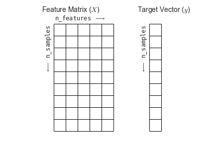
It is very important to understand that Xtrain must be in the form of a 2x2 array with each row corresponding to one sample, and each column corresponding to the feature values for that sample.
ytrain on the other hand is a simple array of responses. These are continuous for regression problems.
Practice with sklearn and a real dataset
We begin by loading up the mtcars dataset. This data was extracted from the 1974 Motor Trend US magazine, and comprises of fuel consumption and 10 aspects of automobile design and performance for 32 automobiles (1973–74 models). We will load this data to a dataframe with 32 observations on 11 (numeric) variables. Here is an explanation of the features:
mpgis Miles/(US) galloncylis Number of cylinders,dispis Displacement (cu.in.),hpis Gross horsepower,dratis Rear axle ratio,wtis the Weight (1000 lbs),qsecis 1/4 mile time,vsis Engine (0 = V-shaped, 1 = straight),amis Transmission (0 = automatic, 1 = manual),gearis the Number of forward gears,carbis Number of carburetors.
import pandas as pd

#load mtcars
dfcars = pd.read_csv("../data/mtcars.csv")
dfcars.head()
# Fix the column title
dfcars = dfcars.rename(columns={"Unnamed: 0":"car name"})
dfcars.head()
dfcars.shape
Searching for values: how many cars have 4 gears?
len(dfcars[dfcars.gear == 4].drop_duplicates(subset='car name', keep='first'))
Next, let's split the dataset into a training set and test set.
# split into training set and testing set
from sklearn.model_selection import train_test_split

#set random_state to get the same split every time
traindf, testdf = train_test_split(dfcars, test_size=0.2, random_state=42)
# testing set is around 20% of the total data; training set is around 80%
print("Shape of full dataset is: {0}".format(dfcars.shape))
print("Shape of training dataset is: {0}".format(traindf.shape))
print("Shape of test dataset is: {0}".format(testdf.shape))
Now we have training and test data. We still need to select a predictor and a response from this dataset. Keep in mind that we need to choose the predictor and response from both the training and test set. You will do this in the exercises below. However, we provide some starter code for you to get things going.
traindf.head()
# Extract the response variable that we're interested in
y_train = traindf.mpg
y_train
Use slicing to get the same vector y_train
Now, notice the shape of y_train.
y_train.shape, type(y_train)
Array reshape
This is a 1D array as should be the case with the Y array. Remember, sklearn requires a 2D array only for the predictor array. You will have to pay close attention to this in the exercises later. Sklearn doesn't care too much about the shape of y_train.
The whole reason we went through that whole process was to show you how to reshape your data into the correct format.
IMPORTANT: Remember that your response variable ytrain can be a vector but your predictor variable xtrain must be an array!
5 - Example: Simple linear regression with automobile data
We will now use sklearn to predict automobile mileage per gallon (mpg) and evaluate these predictions. We already loaded the data and split them into a training set and a test set.
We need to choose the variables that we think will be good predictors for the dependent variable mpg.
- Pick one variable to use as a predictor for simple linear regression. Discuss your reasons with the person next to you.
- Justify your choice with some visualizations.
- Is there a second variable you'd like to use? For example, we're not doing multiple linear regression here, but if we were, is there another variable you'd like to include if we were using two predictors?
x_wt = dfcars.wt
x_wt.shape
# Your code here
# %load solutions/cars_simple_EDA.py
y_mpg = dfcars.mpg
x_wt = dfcars.wt
x_hp = dfcars.hp

fig_wt, ax_wt = plt.subplots(1,1, figsize=(10,6))
ax_wt.scatter(x_wt, y_mpg)
ax_wt.set_xlabel(r'Car Weight')
ax_wt.set_ylabel(r'Car MPG')

fig_hp, ax_hp = plt.subplots(1,1, figsize=(10,6))
ax_hp.scatter(x_hp, y_mpg)
ax_hp.set_xlabel(r'Car HP')
ax_hp.set_ylabel(r'Car MPG')


- Use
sklearnto fit the training data using simple linear regression. - Use the model to make mpg predictions on the test set.
- Plot the data and the prediction.
- Print out the mean squared error for the training set and the test set and compare.
from sklearn.linear_model import LinearRegression
from sklearn.model_selection import train_test_split
from sklearn.metrics import mean_squared_error

dfcars = pd.read_csv("../data/mtcars.csv")
dfcars = dfcars.rename(columns={"Unnamed: 0":"name"})

dfcars.head()
traindf, testdf = train_test_split(dfcars, test_size=0.2, random_state=42)

y_train = np.array(traindf.mpg)
X_train = np.array(traindf.wt)
X_train = X_train.reshape(X_train.shape[0], 1)
y_test = np.array(testdf.mpg)
X_test = np.array(testdf.wt)
X_test = X_test.reshape(X_test.shape[0], 1)
# Let's take another look at our data
dfcars.head()
# And out train and test sets
y_train.shape, X_train.shape
y_test.shape, X_test.shape
#create linear model
regression = LinearRegression()

#fit linear model
regression.fit(X_train, y_train)

predicted_y = regression.predict(X_test)

r2 = regression.score(X_test, y_test)
print(f'R^2 = {r2:.5}')
print(regression.score(X_train, y_train))

print(mean_squared_error(predicted_y, y_test))
print(mean_squared_error(y_train, regression.predict(X_train)))

print('Coefficients: \n', regression.coef_[0], regression.intercept_)
fig, ax = plt.subplots(1,1, figsize=(10,6))
ax.plot(y_test, predicted_y, 'o')
grid = np.linspace(np.min(dfcars.mpg), np.max(dfcars.mpg), 100)
ax.plot(grid, grid, color="black") # 45 degree line
ax.set_xlabel("actual y")
ax.set_ylabel("predicted y")

fig1, ax1 = plt.subplots(1,1, figsize=(10,6))
ax1.plot(dfcars.wt, dfcars.mpg, 'o')
xgrid = np.linspace(np.min(dfcars.wt), np.max(dfcars.wt), 100)
ax1.plot(xgrid, regression.predict(xgrid.reshape(100, 1)))


6 - $k$-nearest neighbors
Now that you're familiar with sklearn, you're ready to do a KNN regression.
Sklearn's regressor is called sklearn.neighbors.KNeighborsRegressor. Its main parameter is the number of nearest neighbors. There are other parameters such as the distance metric (default for 2 order is the Euclidean distance). For a list of all the parameters see the Sklearn kNN Regressor Documentation.
Let's use $5$ nearest neighbors.
# Import the library
from sklearn.neighbors import KNeighborsRegressor
# Set number of neighbors
k = 5
knnreg = KNeighborsRegressor(n_neighbors=k)
# Fit the regressor - make sure your numpy arrays are the right shape
knnreg.fit(X_train, y_train)

# Evaluate the outcome on the train set using R^2
r2_train = knnreg.score(X_train, y_train)

# Print results
print(f'kNN model with {k} neighbors gives R^2 on the train set: {r2_train:.5}')
knnreg.predict(X_test)
Calculate and print the $R^{2}$ score on the test set
# Your code here
Not so good? Lets vary the number of neighbors and see what we get.
# Make our lives easy by storing the different regressors in a dictionary
regdict = {}

# Make our lives easier by entering the k values from a list
k_list = [1, 2, 4, 15]

# Do a bunch of KNN regressions
for k in k_list:
    knnreg = KNeighborsRegressor(n_neighbors=k)
    knnreg.fit(X_train, y_train)
    # Store the regressors in a dictionary
    regdict[k] = knnreg

# Print the dictionary to see what we have
regdict
Now let's plot all the k values in same plot.
fig, ax = plt.subplots(1,1, figsize=(10,6))

ax.plot(dfcars.wt, dfcars.mpg, 'o', label="data")

xgrid = np.linspace(np.min(dfcars.wt), np.max(dfcars.wt), 100)

# let's unpack the dictionary to its elements (items) which is the k and Regressor
for k, regressor in regdict.items():
    predictions = regressor.predict(xgrid.reshape(-1,1))
    ax.plot(xgrid, predictions, label="{}-NN".format(k))

ax.legend();

Explain what you see in the graph. Hint Notice how the $1$-NN goes through every point on the training set but utterly fails elsewhere.
Lets look at the scores on the training set.
ks = range(1, 15) # Grid of k's
scores_train = [] # R2 scores
for k in ks:
    # Create KNN model
    knnreg = KNeighborsRegressor(n_neighbors=k)

    # Fit the model to training data
    knnreg.fit(X_train, y_train)

    # Calculate R^2 score
    score_train = knnreg.score(X_train, y_train)
    scores_train.append(score_train)

# Plot
fig, ax = plt.subplots(1,1, figsize=(12,8))
ax.plot(ks, scores_train,'o-')
ax.set_xlabel(r'$k$')
ax.set_ylabel(r'$R^{2}$')

- Why do we get a perfect $R^2$ at k=1 for the training set?
- Make the same plot as above on the test set.
- What is the best $k$?
# Your code here
# %load solutions/knn_regression.py
ks = range(1, 7) # Grid of k's
scores_test = [] # R2 scores
for k in ks:
    knnreg = KNeighborsRegressor(n_neighbors=k) # Create KNN model
    knnreg.fit(X_train, y_train) # Fit the model to training data
    score_test = knnreg.score(X_test, y_test) # Calculate R^2 score
    scores_test.append(score_test)

# Plot
fig, ax = plt.subplots(1,1, figsize=(12,8))
ax.plot(ks, scores_test,'o-', ms=12)
ax.set_xlabel(r'$k$')
ax.set_ylabel(r'$R^{2}$')

# solution to previous exercise
r2_test = knnreg.score(X_test, y_test)
print(f'kNN model with {k} neighbors gives R^2 on the test set: {r2_test:.5}')