Lab 4: Optimal Number of Clusters

Key Word(s): Elbow Plot, Silhouette, DBSCAN

Some parts of this lab are inspired by Ryan Tibshirani's course Data Mining at Carnegie Mellon University

Choosing the Optimal Number of Clusters

In most exploratory applications, the number of clusters $K$ is unknown. Determining the number of clusters is a very difficult problem. We can not visually determine the number of clusters unless the data are low-dimensional. It's also hard to quantify exactly what makes a cluster and why one clustering scheme is better than another.

The number of clusters is highly dependent on which clustering method you choose and how you decide to choose the correct number of clusters. There is no 100% correct answer.

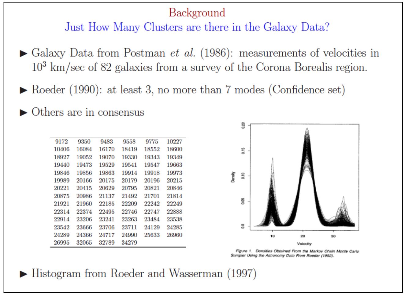
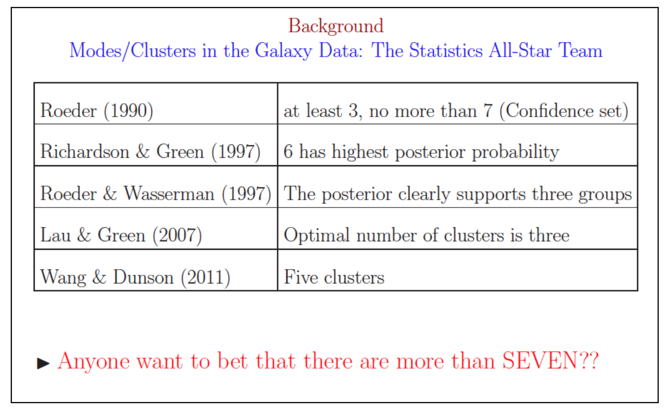
Galaxy Clusters Example

(George Cassella 2011) Looking at a single patch of the sky, it is difficult to determine which galaxies are part of the same cluster and which are not. Astronomers use the relative galaxy velocity to create clusters from the observations. It would be useful to know exactly how many galaxy clusters wer are looking for in our patch of sky.

The result: over 10 years of trying to determine the number of exact clusters and many different answers.

Cassella 1

Cassella 2

Methods to Choose the Optimal Number of Clusters

Here we will go through the methods that Mark mentioned in class. Let's revisit our civil war dataset:

#install.packages('cluster.datasests')
library(cluster.datasets)
library(ggfortify)

# Load Data
data(us.civil.war.battles)
?us.civil.war.battles

# Seperate the names for later
civilWar<-us.civil.war.battles[,-1]
rownames(civilWar)<-us.civil.war.battles[,1]


# Plot PCs
cw.pca<-prcomp(civilWar,scale=F,center=F)

autoplot(cw.pca)+
  geom_density2d()+
  ggtitle('First 2 PCs of Civil War Data')

Elbow Plot

The elbow method looks at the within-cluster sum of squared distances between all pairs of cluster $k$. Note that the within cluster sum of squared distances decreases when we increase $k$. Instead of looking for an extrema, we look for an elbow in the plot.

library(NbClust)
library(factoextra)

fviz_nbclust(civilWar,kmeans,method='wss')+
  ggtitle('K-means clustering for Civil War Data')

Based on the elbow plot, we decide to divide the civil war data into 2 clusters, though 5 also looks like a possible split.

Average Silhouette

The silhouette measures the difference between the dissimilarity between observation $i$ and other points in the next clostest cluster and other points in the cluster in which $i$ belongs to. Here we look at the average silhouette statistic across clusters. It is intuitive that we want to maximize this value.

fviz_nbclust(civilWar,kmeans,method='silhouette')+
  ggtitle('K-means clustering for Civil War Data - Silhouette Method')

Again we see that the optimal number of clusters is 2 according to this method.

Gap Statistic

When the Gap method chooses 1 cluster as optimal, there is insufficient evidence to suggest that any clusters exist.

library(cluster)
set.seed(333)

cw.gap<-clusGap(civilWar,FUN=kmeans,K.max=10,B=500,d.power=2)
fviz_gap_stat(cw.gap,
              maxSE=list(method='Tibs2001SEmax',SE.factor=1))

The optimal number of clusters determined by the Gap statistic is 2.

Aggregate

Since there is no best way of choosing the number of clusters, we can aggregate over all of them and see which is most commonly chosen.

cw.agg<-NbClust(scale(civilWar),method='kmeans',index='alllong')
#Data needs to be scaled for some methods
fviz_nbclust(cw.agg) + theme_minimal()

Most of the methods choose 2. Let's re-fit our k-means so that $k=2$.

cw.kmeans<-kmeans(civilWar,2)
fviz_cluster(cw.kmeans,data=civilWar)

Bayesian Inference Criterion Using `Mclust`

The Mclust function determines the optimal number of clusterst according to the Bayesian Inference Criterion (BIC):

$$ \mbox{BIC} = \ln (n) \omega -2 \ln (\hat L) $$ Where $\hat L$ is the maximized likelihood function and $\omega$ is the number of parameters estimated in the model. Typically, we want to minimized this criterion. Th function Mclust does this for you if you specify multiple clusters (default is 1 through 9):

library(mclust)
cw.mclust<-Mclust(civilWar)
cw.mclust$G
fviz_cluster(cw.mclust,frame.type='norm',geom='point')

Checking Your Clusters

Clusters are well dispersed. i.e. you don't want all ponts but one or two to be in a single cluster as this is an indication that your method is too sensative to outliers or that no cluster actually exists.
Silhouette plot quantifies whether an observation is correctly assigned to a clsuter or not.
$s \approx 1$ - well clustered
$s \approx 0$ - lie between two clusters
$s<0$ - probably in the wrong cluster

fviz_silhouette(silhouette(cw.kmeans$cluster,dist=daisy(civilWar,metric='euclidean')),main='Silhouette plot for Kmeans Clustering')

It appears that most of the observations in cluster 2 are a good fit. Many observations in cluster 1 closely resemble those in cluster 2. None appear to be incorrectly assigned to a cluster.

Your Turn: Find the Optimal Number of Clusters for Trump Tweets

Last time we assumed that there were only two clusters, yet there was visual evidence to suggest that there may be more than 2 clusters. We will use the numerical data to explore the optimal number of clusters for k-medoids clustering. Just like the galaxy example, the clustering method will dictate the optimal number clusters.

First lets load the data from last time. I gave it to you pre-formatted.

load('trumpTweet_2017.Rdata')
# Var name 'tweets'

cl.vars <- c("retweet_count","favorite_count", "source", "day", "weekday", "time", "hashes", "mentions", "link")
num.vars <- c("retweet_count", "favorite_count", "day", "weekday",
              "time", "hashes", "mentions")

For the parts below use only the numerical data to create clusters via PAM using a manhattan distance metric.

tweet.num<-tweets[num.vars]

Using the elbow method, what is the optimal number of clusters?

Using the silhouette method, what is the optimal number of clusters?

Interpret the graph created via the gap statistic method. What is the optimal number of clusters?

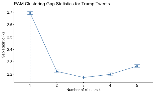
We must set d.power=2 in the function clusGap() and method='Tibs2001SEmax' in the function fviz_gap_stat() to use the same GAP method mark used in class.

#gapstat.pam=clusGap(scale(tweet.num),FUN=pam,K.max=10,d.power=2,B=500,metric='manhattan')

#png('gapTrump_num.png',width=500,height=300)
#fviz_gap_stat(gapstat.pam,
#              maxSE=list(method='Tibs2001SEmax',SE.factor=1))+
#  ggtitle('PAM Clustering Gap Statistics for Trump Tweets')
# dev.off()

Use the NbClust function in the NbClust library to aggregate results across all the clustering functions? (Hint: use index='all' or 'alllong')

```{r,error=T}

Normally we would use 'all' or 'alllong' for the index, but there is a bug in one of the methods so we cannot run all of them. Run all the models in the inds vector below.

This takes a few minutes to run.

inds <- c("kl", "ch", "hartigan", "ccc", "scott", "marriot", "trcovw", "tracew", "friedman", "rubin", "cindex", "db", "silhouette", "duda", "pseudot2", "ratkowsky", "ball", "ptbiserial", "mcclain", "dunn", "hubert", "sdindex", "dindex", "sdbw") inds.k<-c() for(ii in inds){

## FINISH THIS LINE HERE tweets.nbc<- #####

cat("index = ", ii, ":\n")
cat("index values:\n")
print(tweets.nbc$All.index)
cat("best cluster number:\n")
print(tweets.nbc$Best.nc)

inds.k&lt;-c(inds.k,tweets.nbc$Best.nc[1])

}

ggplot(data.frame(k=inds.k),aes(x=k))+ geom_bar()

5.  Based on the results from above, what is the optimal number of clusters for K-mediods clustering? Run k-medoids clustering using the optimal number of clusters $K$ and visualized your results.



```{r}

Use a silhouette plot to determine if any observations were missclustered.

(Advanced aka if you have time) For the parts below use the numerical and categorical data to create clusters via Agglomerative clustering with the "ward" method.

Here is what agg. clustering gives with two clusters:

library(cluster)
library(ggplot2)
tweet.cat<-tweets[cl.vars]
tweets.dist.cat <- daisy(tweet.cat,
                     metric = "gower",stand=T)
tweets.mds <- data.frame(tweet.cat,cmdscale(tweets.dist.cat))

tweet.agnes<-agnes(tweets.dist.cat,diss=T,method='ward')
grp.agnes<-cutree(tweet.agnes,k=2)
tweet.agnes.df<-data.frame(tweets.mds,cluster=factor(grp.agnes))
ggplot(tweet.agnes.df,
       mapping = aes(x = X1,
                     y = X2,col=cluster)) +
    geom_point()

Note that using categorical factors limit the methods we are able to use to determine the optimal number of clusters. Out of the Elbow, Average Silhouette, and Gap Statistics methods R is only able to apply Average Silhouette.

Using the silhouette method, what is the optimal number of clusters?

Use the NbClust function in the NbClust library to aggregate results across all the clustering functions? Using the NbClust function with only a distance matrix we are able to use a subset of the indexes: frey,mcclain,cindex,silhouette, and dunn.

Based on the results from above, what is the optimal number of clusters for K-mediods clustering? Run k-medoids clustering using the optimal number of clusters $K$ and visualized your results.

Density-Based Clustering Algorithm

Applied in R using the dbscan function. Mark highlighted some huge advantages using this algorithm in class.

In order to estimate $\epsilon$ use kNNdistplot in the dbscan package.

library(dbscan)
kNNdistplot(scale(tweet.num),k=2)
abline(h=2.2,lwd=2,col='red',lty=3)
abline(h=1.2,lwd=2,col='red',lty=3)

Next we implement dbscan using the epsilon determined above:

tweet.db<-dbscan(scale(tweet.num),eps=2,minPts = 8)
fviz_cluster(tweet.db,data=scale(tweet.num),geom='point')

table(tweet.db$cluster)

Your Turn: Explore DBScan

Create an average silhouette plot using your DB Scan results.

Do you think this data set is a good fit for Density Based Clustering? Why or why not?