CS109A/STAT121A Introduction to Data Science

Lab 3: `numpy`, plotting, K-NN Regression, Simple Linear Regression¶

PRE-LAB : DO THIS PART BEFORE COMING TO LAB¶

Harvard University
Fall 2018
Instructors: Pavlos Protopapas and Kevin Rader

Material prepared by: David Sondak, Will Claybaugh and Pavlos Protopapas

In [ ]:

#RUN THIS CELL 
import requests
from IPython.core.display import HTML
styles = requests.get("https://raw.githubusercontent.com/Harvard-IACS/2018-CS109A/master/content/styles/cs109.css").text
HTML(styles)

Table of Contents¶

A revision of `numpy`
A revision of matplotlib - Creating plots

1 - Numerical Python: `numpy`¶

Review the concepts on numpy: Scientific Python code uses a fast array structure, called the numpy array. Those who have worked in Matlab will find this very natural. For reference, the numpy documention can be found here: numpy.

Let's make a numpy array.

In [ ]:

import numpy as np

In [ ]:

my_array = np.array([1,4,9,16])
my_array

Numpy arrays support the same operations as lists! Below we compute length, slice, and iterate.

In [ ]:

print("len(array):", len(my_array)) # Length of array

print("array[2:4]:", my_array[2:4]) # A slice of the array

# Iterate over the array
for ele in my_array:
    print("element:", ele)

In general you should manipulate numpy arrays by using numpy module functions (e.g. np.mean). This is for efficiency purposes, and a discussion follows below this section.

You can calculate the mean of the array elements either by calling the method .mean on a numpy array or by applying the function np.mean with the numpy array as an argument.

In [ ]:

# Two ways of calculating the mean

print(my_array.mean())

print(np.mean(my_array))

The way we constructed the numpy array above seems redundant. After all we already had a regular python list. Indeed, it is the other ways we have to construct numpy arrays that make them super useful.

There are many such numpy array constructors. Here are some commonly used constructors. Look them up in the documentation.

In [ ]:

zeros = np.zeros(10) # generates 10 floating point zeros
zeros

Numpy gains a lot of its efficiency from being strongly typed. That is, all elements in the array have the same type, such as integer or floating point. The default type, as can be seen above, is a float of size appropriate for the machine (64 bit on a 64 bit machine).

In [ ]:

zeros.dtype

In [ ]:

np.ones(10, dtype='int') # generates 10 integer ones

If the elements of an array are of a different type, numpy will force them into the same type (the longest in terms of bytes)

In [ ]:

mixed = np.array([1, 2.3, 'eleni', True])

#elements are of different type
print(type(1), type(2.3), type('eleni'), type(True))

# all elements will become strings
mixed

Often you will want random numbers. Use the random constructor!

In [ ]:

np.random.rand(10) # uniform on [0,1]

You can generate random numbers from a normal distribution with mean $0$ and variance $1$ using np.random.randn:

In [ ]:

normal_array = np.random.randn(10000)
print("The sample mean and standard devation are {0:17.16f} and {1:17.16f}, respectively.".format(np.mean(normal_array), np.std(normal_array)))

`numpy` supports vector operations¶

What does this mean? It means that to add two arrays instead of looping ovr each element (e.g. via a list comprehension as in base Python) you get to simply put a plus sign between the two arrays.

In [ ]:

ones_array = np.ones(5)
twos_array = 2*np.ones(5)
ones_array + twos_array

Note that this behavior is very different from python lists, which just get longer when you try to + them.

In [ ]:

first_list = [1., 1., 1., 1., 1.]
second_list = [2., 2., 2., 2., 2.]
first_list + second_list # not what you want

On some computer chips nunpy's addition actually happens in parallel, so speedups can be high. But even on regular chips, the advantage of greater readability is important.

Numpy supports a concept known as broadcasting, which dictates how arrays of different sizes are combined together. There are too many rules to list all of them here. Here are two important rules:

Multiplying an array by a number multiplies each element by the number
Adding a number adds the number to each element.

In [ ]:

ones_array + 1

In [ ]:

5 * ones_array

This means that if you wanted the distribution $N(5, 7)$ you could do:

In [ ]:

normal_5_7 = 5.0 + 7.0 * normal_array

np.mean(normal_5_7), np.std(normal_5_7)

Now you have seen how to create and work with simple one dimensional arrays in numpy. You have also been introduced to some important numpy functionality (e.g. mean and std).

Next, we push ahead to two-dimensional arrays and begin to dive into some of the deeper aspects of numpy.

2D arrays¶

We can create two-dimensional arrays without too much fuss.

In [ ]:

# create a 2d-array by handing a list of lists
my_array2d = np.array([ 
    [1, 2, 3, 4], 
    [5, 6, 7, 8], 
    [9, 10, 11, 12] 
])

# you can do the same without the pretty formatting (decide which style you like better)
my_array2d = np.array([ [1, 2, 3, 4], [5, 6, 7, 8], [9, 10, 11, 12] ])


# 3 x 4 array of ones
ones_2d = np.ones([3, 4])
print(ones_2d, "\n")

# 3 x 4 array of ones with random noise
ones_noise = ones_2d + 0.01*np.random.randn(3, 4)
print(ones_noise, "\n")

# 3 x 3 identity matrix
my_identity = np.eye(3)
print(my_identity, "\n")

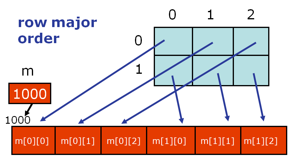
Like lists, numpy arrays are $0$-indexed. Thus we can access the $n$th row and the $m$th column of a two-dimensional array with the indices $[n - 1, m - 1]$.

In [ ]:

print(my_array2d)
print("element [2,3] is:", my_array2d[2, 3])

Numpy arrays can be sliced, and can be iterated over with loops. Below is a schematic illustrating slicing two-dimensional arrays.

Drawing

Notice that the list slicing syntax still works!
array[2:,3] says "in the array, get rows 2 through the end, column 3]"
array[3,:] says "in the array, get row 3, all columns".

Numpy functions will by default work on the entire array:

In [ ]:

np.sum(ones_2d)

The axis 0 is the one going downwards (i.e. the rows), whereas axis 1 is the one going across (the columns). You will often use functions such as mean or sum along a particular axis. If you sum along axis 0 you are summing across the rows and will end up with one value per column. As a rule, any axis you list in the axis argument will dissapear.

In [ ]:

np.sum(ones_2d, axis=0)

In [ ]:

np.sum(ones_2d, axis=1)

Exercise

Create a two-dimensional array of size $3\times 5$ and do the following:
- Print out the array
- Print out the shape of the array
- Create two slices of the array:
  1. The first slice should be the last row and the third through last column
  2. The second slice should be rows $1-3$ and columns $3-5$
- Square each element in the array and print the result

In [ ]:

# your code here
A = np.array([ [5, 4, 3, 2, 1], [1, 2, 3, 4, 5], [1.1, 2.2, 3.3, 4.4, 5.5] ])
print(A, "\n")

# set length(shape)
dims = A.shape
print(dims, "\n")

# slicing
print(A[-1, 2:], "\n")
print(A[1:3, 3:5], "\n")

# squaring
A2 = A * A
print(A2)

`numpy` supports matrix operations¶

2d arrays are numpy's way of representing matrices. As such there are lots of built-in methods for manipulating them

Earlier when we generated the one-dimensional arrays of ones and random numbers, we gave ones and random the number of elements we wanted in the arrays. In two dimensions, we need to provide the shape of the array, i.e., the number of rows and columns of the array.

In [ ]:

three_by_four = np.ones([3,4])
three_by_four

You can transpose the array:

In [ ]:

three_by_four.shape

In [ ]:

four_by_three = three_by_four.T

In [ ]:

four_by_three.shape

Matrix multiplication is accomplished by np.dot. The * operator will do element-wise multiplication.

In [ ]:

print(np.dot(three_by_four, four_by_three)) # 3 x 3 matrix
np.dot(four_by_three, three_by_four) # 4 x 4 matrix

Numpy has functions to do the difficult matrix operations that are awful to do by hand.

In [ ]:

matrix = np.random.rand(4,4) # a 4 by 4 matrix
matrix

Let's get the eigenvalues and eigenvectors!

In [ ]:

np.linalg.eig(matrix)

How about inverses?

In [ ]:

inv_matrix = np.linalg.inv(matrix) # the invert matrix
print(inv_matrix)

#prove it's the inverse
np.dot(matrix,inv_matrix)

Notice that there is a bit of 'rounding error' in the inverse calculation. This is becuase the computer can't store the exact values the inverse matrix asks for (they have more decimal places than the computer can hold). Built-in numpy routines manage these errors, which is why it's very important to use pre-built tools whenever possible, and to be very cautious when writing your own.

(It happens that there are even more advanced numpy functions like np.linalg.solve which are more accurate than just taking the naked inverse)

See the documentation to learn more about numpy functions as needed.

Numpy's layout in the computer's memory¶

Advanced coders: You should notice that access is row-by-row and one dimensional iteration gives a row. This is because numpy lays out memory row-wise.

Starting coders: If you really need a particular section of numpy to run faster, ask an advanced coder to point out improvements in your code. They may have you transpose your arrays. But if your code is fast enough, then it's fast enough.

Drawing

(from https://aaronbloomfield.github.io)

An often seen idiom allocates a two-dimensional array, and then fills in one-dimensional arrays from some function. We will discuss why this is a bad design pattern.

In [ ]:

# allocate a 2D array
twod = np.zeros([5, 2])
print(twod, "\n")

# Fill in with random numbers
for i in range(twod.shape[0]):
    twod[i, :] = np.random.random(2)
print(twod)

In this and many other cases, it is faster to simply do:

In [ ]:

twod = np.random.random(size=(5,2))
twod

`Numpy`Arrays vs. `Python` Lists?¶

Why the need for numpy arrays? Can't we just use Python lists?
Iterating over numpy arrays is slow. Slicing is faster.

Python lists may contain items of different types. This flexibility comes at a price: Python lists store pointers to memory locations. On the other hand, numpy arrays are typed, where the default type is floating point. Because of this, the system knows how much memory to allocate, and if you ask for an array of size $100$, it will allocate one hundred contiguous spots in memory, where the size of each spot is based on the type. This makes access extremely fast.

Drawing

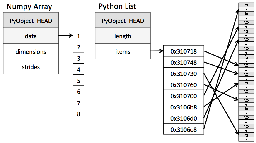
(image from Jake Vanderplas's Data Science Handbook)

Unfortunately, looping over an array slows things down. In general you should not access numpy array elements by iteration. This is because of type conversion. Numpy stores integers and floating points in C-language format. When you operate on array elements through iteration, Python needs to convert that element to a Python int or float, which is a more complex beast (a struct in C jargon). This has a cost.

Drawing

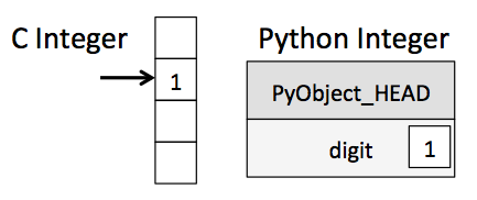
(image from Jake Vanderplas's Data Science Handbook)

If you want to know more, we will suggest that you read

Jake Vanderplas's Data Science Handbook.
Wes McKinney's Python for Data Analysis (HOLLIS)
You will find them both incredible resources for this class.

Why is slicing faster? The reason is technical: slicing provides a view onto the memory occupied by a numpy array, instead of creating a new array. That is the reason the code above this cell works nicely as well. However, if you iterate over a slice, then you have gone back to the slow access.

By contrast, functions such as np.dot are implemented at C-level, do not do this type conversion, and access contiguous memory. If you want this kind of access in Python, use the struct module or Cython. Indeed many fast algorithms in numpy, pandas, and C are either implemented at the C-level, or employ Cython.

Concept Check:¶

Answer these questions and see the bottom of the lab to check your answers.

What is the major benefit of working in numpy?
Why is it vital to use built-in numpy functions whenever possible?
You need to find the running total of each element in a numpy array. For example, the input [2,5,3,2] should give the output [2,7,10,12]. Rather than writing your own code, think of at least two google querrys to find a relevant numpy function.
What numpy function does the job above?

2 - Plotting with matplot lib (and beyond)¶

Conveying your findings convincingly is an absolutely crucial part of any analysis. Therefore, you must be able to write well and make compelling visuals. Creating informative visuals is an involved process and we won't cover that in this lab. However, part of creating informative data visualizations means generating readable figures. If people can't read your figures or have a difficult time interpreting them, they won't understand the results of your work. Here are some non-negotiable commandments for any plot:

Label $x$ and $y$ axes
Axes labels should be informative
Axes labels should be large enough to read
Make tick labels large enough
Include a legend if necessary
Include a title if necessary
Use appropriate line widths
Use different line styles for different lines on the plot
Use different markers for different lines

There are other important elements, but that list should get you started on your way.

Here is the anatomy of a figure: Drawing

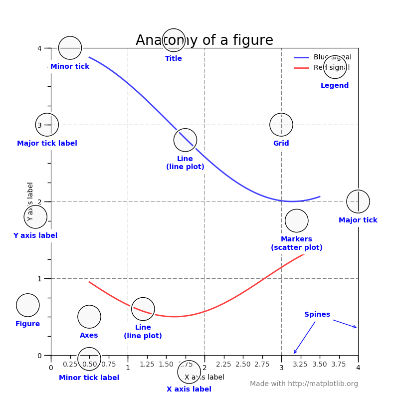
taken from showcase example code: anatomy.py.

We will work with matplotlib and seaborn for plotting in this class. Today's lab will focus on matplotlib, which is a very powerful python library for making scientific plots. seaborn is a little more specialized in that it was developed for statistical data visualization. We will put in a little bit of seaborn at the end, but if you are comfortable with matplotlib then seaborn will be a breeze.

Before diving in, one more note should be made. We will not focus on the internal aspects of matplotlib. Today's lab will really only focus on the basics and developing good plotting practices. There are many excellent tutorials out there for matplotlib. For example,

Okay, let's get started!

`matplotlib`¶

First, let's generate some data.

Exercise

Use the following three functions to make some plots:

Logistic function: \begin{align*} f\left(z\right) = \dfrac{1}{1 + be^{-az}} \end{align*} where $a$ and $b$ are parameters.
Hyperbolic tangent: \begin{align*} g\left(z\right) = b\tanh\left(az\right) + c \end{align*} where $a$, $b$, and $c$ are parameters.
Rectified Linear Unit: \begin{align*} h\left(z\right) = \left{
```
\begin{array}{lr}
  z, \quad z > 0 \\
  \epsilon z, \quad z\leq 0
\end{array}
```
\right. \end{align*} where $\epsilon < 0$ is a small, positive parameter.

You are given the code for the first two functions. Notice that $z$ is passed in as a numpy array and that the functions are returned as numpy arrays. Parameters are passed in as floats.

You should write a function to compute the rectified linear unit. The input should be a numpy array for $z$ and a positive float for $\epsilon$.

In [ ]:

# Your code here
import numpy as np

def logistic(z: np.ndarray, a: float, b: float) -> np.ndarray:
    """ Compute logistic function
      Inputs:
         a: exponential parameter
         b: exponential prefactor
         z: numpy array; domain
      Outputs:
         f: numpy array of floats, logistic function
    """
    
    den = 1.0 + b * np.exp(-a * z)
    return 1.0 / den

def stretch_tanh(z: np.ndarray, a: float, b: float, c: float) -> np.ndarray:
    """ Compute stretched hyperbolic tangent
      Inputs:
         a: horizontal stretch parameter (a>1 implies a horizontal squish)
         b: vertical stretch parameter
         c: vertical shift parameter
         z: numpy array; domain
      Outputs:
         g: numpy array of floats, stretched tanh
    """
    return b * np.tanh(a * z) + c

def relu(z: np.ndarray, eps: float = 0.01) -> np.ndarray:
    """ Compute rectificed linear unit
      Inputs:
         eps: small positive parameter
         z: numpy array; domain
      Outputs:
         h: numpy array; relu
    """
    return np.fmax(z, eps * z)

Now let's make some plots. First, let's just warm up and plot the logistic function.

In [ ]:

x = np.linspace(-5.0, 5.0, 100) # Equally spaced grid of 100 pts between -5 and 5

f = logistic(x, 1.0, 1.0) # Generate data

In [ ]:

import matplotlib.pyplot as plt

# This is only needed in Jupyter notebooks!  Displays the plots for us.
%matplotlib inline 

plt.plot(x, f); # Use the semicolon to suppress some iPython output (not needed in real Python scripts)

Wonderful! We have a plot. It's terribly ugly and uninformative. Let's clean it up a bit by putting some labels on it.

In [ ]:

plt.plot(x, f)
plt.xlabel('x')
plt.ylabel('f')
plt.title('Logistic Function');

Okay, it's getting better. Still super ugly. I see these kinds of plots at conferences all the time. Unreadable. We can do better. Much, much better. First, let's throw on a grid.

In [ ]:

plt.plot(x, f)
plt.xlabel('x')
plt.ylabel('f')
plt.title('Logistic Function')
plt.grid(True)

At this point, our plot is starting to get a little better but also a little crowded.

A note on gridlines¶

Gridlines can be very helpful in many scientific disciplines. They help the reader quickly pick out important points and limiting values. On the other hand, they can really clutter the plot. Some people recommend never using gridlines, while others insist on them being present. The correct approach is probably somewhere in between. Use gridlines when necessary, but dispense with them when they take away more than they provide. Ask yourself if they help bring out some important conclusion from the plot. If not, then best just keep them away.

Before proceeding any further, I'm going to change notation. The plotting interface we've been working with so far is okay, but not as flexible as it can be. In fact, I don't usually generate my plots with this interface. I work with slightly lower-level methods, which I will introduce to you now. The reason I need to make a big deal about this is because the lower-level methods have a slightly different API. This will become apparent in my next example.

In [ ]:

fig, ax = plt.subplots(1,1) # Get figure and axes objects

ax.plot(x, f) # Make a plot

# Create some labels
ax.set_xlabel('x')
ax.set_ylabel('f')
ax.set_title('Logistic Function')

# Grid
ax.grid(True)

Wow, it's exactly the same plot! Notice, however, the use of ax.set_xlabel() instead of plt.xlabel(). The difference is tiny, but you should be aware of it. I will use this plotting syntax from now on.

What else do we need to do to make this figure better? Here are some options:

Make labels bigger!
Make line fatter
Make tick mark labels bigger
Make the grid less pronounced
Make figure bigger

Let's get to it.

In [ ]:

fig, ax = plt.subplots(1,1, figsize=(10,6)) # Make figure bigger

ax.plot(x, f, lw=4) # Linewidth bigger
ax.set_xlabel('x', fontsize=24) # Fontsize bigger
ax.set_ylabel('f', fontsize=24) # Fontsize bigger
ax.set_title('Logistic Function', fontsize=24) # Fontsize bigger
ax.grid(True, lw=1.5, ls='--', alpha=0.75) # Update grid

Notice:

lw stands for linewidth. We could also write ax.plot(x, f, linewidth=4)
ls stands for linestyle.
alpha stands for transparency.

Things are looking good now! Unfortunately, people still can't read the tick mark labels. Let's remedy that presently.

In [ ]:

fig, ax = plt.subplots(1,1, figsize=(10,6)) # Make figure bigger

# Make line plot
ax.plot(x, f, lw=4)

# Update ticklabel size
ax.tick_params(labelsize=24)

# Make labels
ax.set_xlabel(r'$x$', fontsize=24) # Use TeX for mathematical rendering
ax.set_ylabel(r'$f(x)$', fontsize=24) # Use TeX for mathematical rendering
ax.set_title('Logistic Function', fontsize=24)

ax.grid(True, lw=1.5, ls='--', alpha=0.75)

The only thing remaining to do is to change the $x$ limits. Clearly these should go from $-5$ to $5$.

In [ ]:

fig, ax = plt.subplots(1,1, figsize=(10,6)) # Make figure bigger

# Make line plot
ax.plot(x, f, lw=4)

# Set axes limits
ax.set_xlim(x.min(), x.max())

# Update ticklabel size
ax.tick_params(labelsize=24)

# Make labels
ax.set_xlabel(r'$x$', fontsize=24) # Use TeX for mathematical rendering
ax.set_ylabel(r'$f(x)$', fontsize=24) # Use TeX for mathematical rendering
ax.set_title('Logistic Function', fontsize=24)

ax.grid(True, lw=1.5, ls='--', alpha=0.75)

You can play around with figures forever making them perfect. At this point, everyone can read and interpret this figure just fine. Don't spend your life making the perfect figure. Make it good enough so that you can convey your point to your audience. Then save if it for later.

In [ ]:

fig.savefig('logistic.png')

Done! Let's take a look.

Resources¶

If you want to see all the styles available, please take a look at the documentation.

We haven't discussed it yet, but you can also put a legend on a figure. You'll do that in the next exercise. Here are some additional resources:

Legend
Grid

Exercise

Do the following:

Make a figure with the logistic function, hyperbolic tangent, and rectified linear unit.
Use different line styles for each plot
Put a legend on your figure

Here's an example of a figure:

You don't need to make the exact same figure, but it should be just as nice and readable.

In [ ]:

# your code here

# First get the data
f = logistic(x, 2.0, 1.0)
g = stretch_tanh(x, 2.0, 0.5, 0.5)
h = relu(x)

fig, ax = plt.subplots(1,1, figsize=(10,6)) # Create figure object

# Make actual plots
# (Notice the label argument!)
ax.plot(x, f, lw=4, ls='-', label=r'$L(x;1)$')
ax.plot(x, g, lw=4, ls='--', label=r'$\tanh(2x)$')
ax.plot(x, h, lw=4, ls='-.', label=r'$relu(x; 0.01)$')

# Make the tick labels readable
ax.tick_params(labelsize=24)

# Set axes limits to make the scale nice
ax.set_xlim(x.min(), x.max())
ax.set_ylim(h.min(), 1.1)

# Make readable labels
ax.set_xlabel(r'$x$', fontsize=24)
ax.set_ylabel(r'$h(x)$', fontsize=24)
ax.set_title('Activation Functions', fontsize=24)

# Set up grid
ax.grid(True, lw=1.75, ls='--', alpha=0.75)

# Put legend on figure
ax.legend(loc='best', fontsize=24);

fig.savefig('nice_plots.png')

There a many more things you can do to the figure to spice it up. Remember, there must be a tradeoff between making a figure look good and the time you put into it.

The guiding principle should be that your audience needs to easily read and understand your figure.

There are of course other types of figures including, but not limited to,

Scatter plots (you will use these all the time)
Bar charts
Histograms
Contour plots
Surface plots
Heatmaps

There is documentation on each one of these. You should feel comforatable enough with the plotting API now to dig in and make readable, understandable plots.

Before moving on, we will discuss another way to make your plots look good without all the hassle. I'll make a beautiful plot without having to specify annoying arguments every single time.

In [ ]:

import config # User-defined config file
plt.rcParams.update(config.pars) # Update rcParams to make nice plots

# First get the data
f1 = logistic(x, 1.0, 1.0)
f2 = logistic(x, 2.0, 1.0)
f3 = logistic(x, 3.0, 1.0)

fig, ax = plt.subplots(1,1, figsize=(10,6)) # Create figure object

# Make actual plots
# (Notice the label argument!)
ax.plot(x, f1, ls='-', label=r'$L(x;-1)$')
ax.plot(x, f2, ls='--', label=r'$L(x;-2)$')
ax.plot(x, f3, ls='-.', label=r'$L(x;-3)$')

# Set axes limits to make the scale nice
ax.set_xlim(x.min(), x.max())
ax.set_ylim(h.min(), 1.1)

# Make readable labels
ax.set_xlabel(r'$x$')
ax.set_ylabel(r'$h(x)$')
ax.set_title('Logistic Functions')

# Set up grid
ax.grid(True, lw=1.75, ls='--', alpha=0.75)

# Put legend on figure
ax.legend(loc='best')

That's a good-looking plot! Notice that we didn't need to have all those annoying fontsize specifications floating around. If you want to reset the defaults, just use plt.rcdefaults().

Now, how in the world did this work? Obviously, there is something special about the config file. I didn't give you a config file, but the next exercise requires you to create one.

Exercise

Read the matplotlib rcParams section at the following page: Customizing matplotlib
Create your very own config.py file. It should have the following structure:
```
pars = {}
```
You must fill in the pars dictionary yourself. All the possible parameters can be found at the link above. For example, if you want to set a default line width of 4, then you would have
```
pars = {'lines.linewidth': 4}
```
in your config.py file.
Make sure your config.py file is in the same directory as your lab notebook.
Make a plot (similar to the one I made above) using your config file.

`seaborn`¶

Early on in this plotting section, we mentioned seaborn. You can use seaborn to make very nice plots of statistical data. Here is the main website: seaborn: statistical data visualization.

We won't dive deep into seaborn here. It is quite popular in the data science community, but it is ultimately up to you whether or not you choose to use it.

seaborn works great with pandas. It can also be customized easily. Here is the basic seaborn tutorial: Seaborn tutorial.

No Excuses¶

With all of these resourses, there is no reason to have a bad figure. We will take this into account for homework.

CS109A/STAT121A Introduction to Data Science

Lab 3: numpy, plotting, K-NN Regression, Simple Linear Regression¶

PRE-LAB : DO THIS PART BEFORE COMING TO LAB¶

Table of Contents¶

1 - Numerical Python: numpy¶

numpy supports vector operations¶

2D arrays¶

numpy supports matrix operations¶

Numpy's layout in the computer's memory¶

NumpyArrays vs. Python Lists?¶

Concept Check:¶

2 - Plotting with matplot lib (and beyond)¶

matplotlib¶

A note on gridlines¶

Resources¶

seaborn¶

No Excuses¶

Lab 3: `numpy`, plotting, K-NN Regression, Simple Linear Regression¶

1 - Numerical Python: `numpy`¶

`numpy` supports vector operations¶

`numpy` supports matrix operations¶

`Numpy`Arrays vs. `Python` Lists?¶

`matplotlib`¶

`seaborn`¶